### 03.01 Load target data  ----------------------------------------------------
load("data/SickSicker_CalibTargets.RData")
lst_targets <- SickSicker_targetsSick-Sicker Model: LHS Random Search Calibration Exercise
01 Calibration Overview
01.01 Model Description
The calibration is performed for the Sick-Sicker 4-state cohort Markov model, which represents the natural history of a chronic disease.
The model includes four health states:
- Healthy (H)
- Sick (S1)
- Sicker (S2)
- Dead (D)
The following model parameters are calibrated:
p_S1S2: Probability of progression from Sick (S1) to Sicker (S2)
hr_S1: Mortality hazard ratio in the Sick state relative to Healthy
hr_S2: Mortality hazard ratio in the Sicker state relative to Healthy
Calibration targets include:
- Survival (
Surv): Proportion of the cohort alive over time
- Prevalence (
Prev): Proportion of the cohort with disease (Sick + Sicker)
- Proportion Sick (
PropSick): Among diseased individuals, the proportion in the Sick (S1) state
01.02 Calibration Method
Calibration is conducted using a random search strategy based on Latin-Hypercube Sampling (LHS).
Model fit is evaluated using the sum of log-likelihoods across all calibration targets and observed time points. The parameter set that maximizes this goodness-of-fit criterion is selected as the best-fitting solution.
02 Setup
03 Load calibration targets
TARGET 1: Survival (“Surv”)
plotrix::plotCI(x = lst_targets$Surv$time, y = lst_targets$Surv$value,
                ui = lst_targets$Surv$ub,
                li = lst_targets$Surv$lb,
                ylim = c(0, 1),
                xlab = "Time", ylab = "Pr Survive")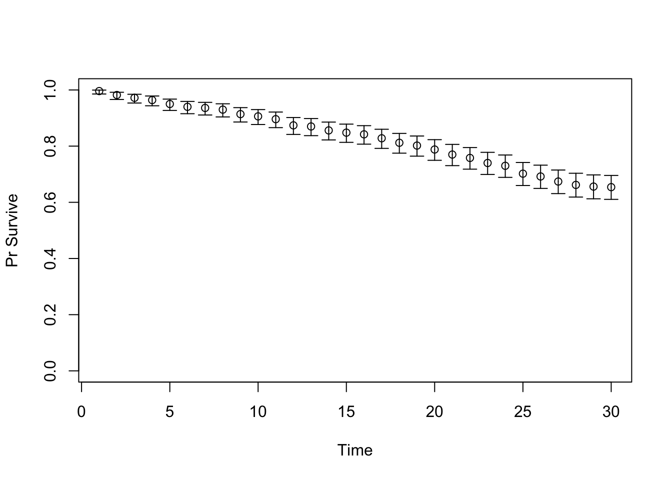
TARGET 2: Prevalence (“Prev”)
plotrix::plotCI(x = lst_targets$Prev$time, y = lst_targets$Prev$value,
                ui = lst_targets$Prev$ub,
                li = lst_targets$Prev$lb,
                ylim = c(0, 1),
                xlab = "Time", ylab = "Prev")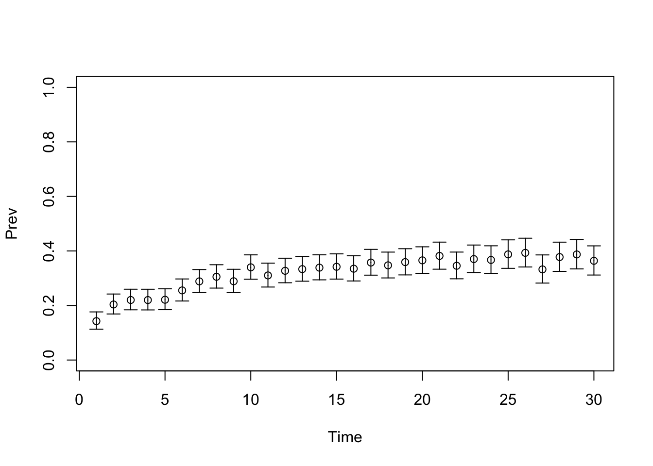
TARGET 3: Proportion who are Sick (“PropSick”), among all those afflicted (Sick+Sicker)
plotrix::plotCI(x = lst_targets$PropSick$time, y = lst_targets$PropSick$value,
                ui = lst_targets$PropSick$ub,
                li = lst_targets$PropSick$lb,
                ylim = c(0, 1),
                xlab = "Time", ylab = "PropSick")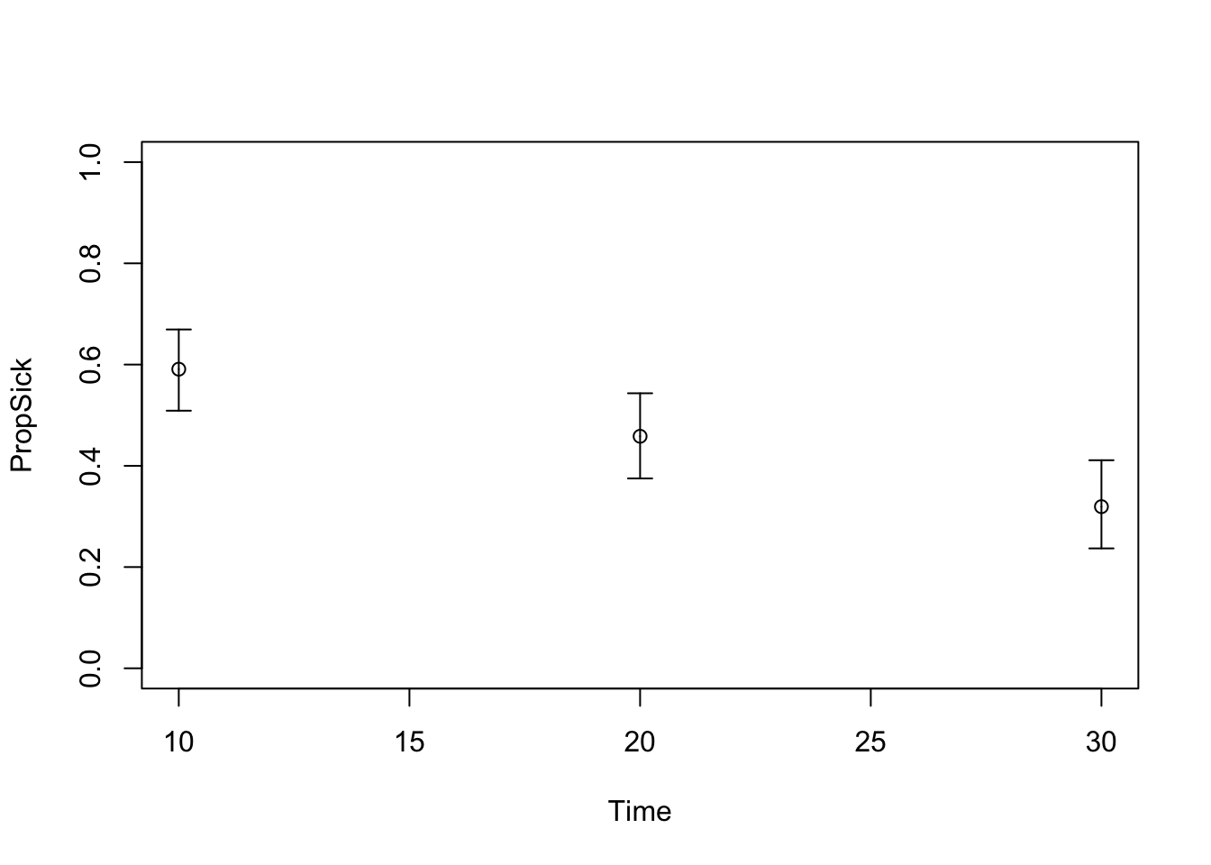
04 Load model as a function
### 04.01 Source model function  -----------------------------------------------
# Function inputs: parameters to be estimated through calibration
# Function outputs: model predictions corresponding to target data
source("code/Functions/SickSicker_MarkovModel_Function.R") # creates the function run_sick_sicker_markov()

### 04.02 Test model function  -------------------------------------------------
v_params_test <- c(p_S1S2 = 0.105, hr_S1 = 3, hr_S2 = 10)
run_sick_sicker_markov(v_params_test) # Test: function works correctly
$Surv
1 2 3 4 5 6 7 8
0.9950000 0.9885362 0.9810784 0.9728008 0.9637994 0.9541472 0.9439082 0.9331413
9 10 11 12 13 14 15 16
0.9219015 0.9102402 0.8982055 0.8858421 0.8731922 0.8602948 0.8471865 0.8339014
17 18 19 20 21 22 23 24
0.8204713 0.8069256 0.7932918 0.7795955 0.7658602 0.7521079 0.7383588 0.7246318
25 26 27 28 29 30
0.7109441 0.6973115 0.6837488 0.6702694 0.6568856 0.6436086
$Prev
1 2 3 4 5 6 7 8
0.1507538 0.2018249 0.2267624 0.2443252 0.2593508 0.2731265 0.2860289 0.2981972
9 10 11 12 13 14 15 16
0.3097057 0.3206084 0.3309506 0.3407725 0.3501104 0.3589973 0.3674630 0.3755352
17 18 19 20 21 22 23 24
0.3832387 0.3905968 0.3976304 0.4043591 0.4108009 0.4169723 0.4228887 0.4285642
25 26 27 28 29 30
0.4340120 0.4392445 0.4442729 0.4491079 0.4537594 0.4582367
$PropSick
10 20 30
0.5372139 0.3734392 0.2997246 05 Calibration specifications
### 05.01 Set random seed  -----------------------------------------------------
set.seed(072218) # For reproducible sequence of random numbers

### 05.02 Define calibration parameters  ---------------------------------------
# number of random samples
n_samp <- 1000

# names and number of input parameters to be calibrated
v_param_names <- c("p_S1S2","hr_S1","hr_S2")
n_param <- length(v_param_names)

# Search space bounds
lb <- c(p_S1S2 = 0.01, hr_S1 = 1.0, hr_S2 = 5) # lower bound
ub <- c(p_S1S2 = 0.50, hr_S1 = 4.5, hr_S2 = 15) # upper bound

### 05.03 Define calibration targets  ------------------------------------------
v_target_names <- c("Surv", "Prev", "PropSick")
n_target <- length(v_target_names)
06 Run calibration using Random Search (LHS)
### 06.01 Record start time  ---------------------------------------------------
t_init <- Sys.time()

### 06.02 Sample input values using Latin Hypercube Sampling  ------------------

# Sample unit Latin Hypercube
m_lhs_unit <- randomLHS(n_samp, n_param)

# Rescale to min/max of each parameter
m_param_samp <- matrix(nrow = n_samp, ncol = n_param)
for (i in 1:n_param) {
  m_param_samp[, i] <- qunif(m_lhs_unit[, i],
                             min = lb[i],
                             max = ub[i])
}
colnames(m_param_samp) <- v_param_names

### 06.03 Visualize parameter samples  -----------------------------------------
pairs.panels(m_param_samp)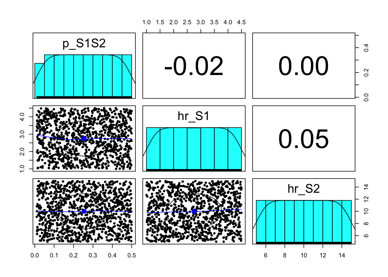
### 06.04 Run the model and calculate goodness-of-fit for each sample  ---------

# initialize goodness-of-fit matrix
m_GOF <- matrix(nrow = n_samp, ncol = n_target)
colnames(m_GOF) <- paste0(v_target_names, "_fit")

# loop through sampled sets of input values
for (j in 1:n_samp) {

  # Run model for a given parameter set
  model_res <- run_sick_sicker_markov(v_params = m_param_samp[j, ])

  # Calculate goodness-of-fit of model outputs to targets

  # TARGET 1: Survival ("Surv") - log likelihood
  m_GOF[j, 1] <- sum(dnorm(x = lst_targets$Surv$value,
                           mean = model_res$Surv,
                           sd = lst_targets$Surv$se,
                           log = T))

  # TARGET 2: "Prev" - log likelihood
  m_GOF[j, 2] <- sum(dnorm(x = lst_targets$Prev$value,
                           mean = model_res$Prev,
                           sd = lst_targets$Prev$se,
                           log = T))

  # TARGET 3: "PropSick" - log likelihood
  m_GOF[j, 3] <- sum(dnorm(x = lst_targets$PropSick$value,
                           mean = model_res$PropSick,
                           sd = lst_targets$PropSick$se,
                           log = T))


} # End loop over sampled parameter sets


### 06.05 Calculate overall GOF  -----------------------------------------------
# can give different targets different weights
v_weights <- matrix(1, nrow = n_target, ncol = 1)
# matrix multiplication to calculate weight sum of each GOF matrix row
v_GOF_overall <- c(m_GOF %*% v_weights)
# Store in GOF matrix with column name "Overall"
m_GOF <- cbind(m_GOF, Overall_fit = v_GOF_overall)

### 06.06 Calculate computation time  ------------------------------------------
comp_time <- Sys.time() - t_init
comp_time
Time difference of 0.1907649 secs07 Explore calibration results
### 07.01 Identify best-fitting parameter sets  --------------------------------
# Arrange parameter sets in order of fit
m_calib_res <- cbind(m_param_samp, m_GOF)
m_calib_res <- m_calib_res[order(-m_calib_res[, "Overall_fit"]), ]

# Examine the top 10 best-fitting sets
m_calib_res[1:10, ]
p_S1S2 hr_S1 hr_S2 Surv_fit Prev_fit PropSick_fit Overall_fit
[1,] 0.07914497 4.081703 10.74360 95.98387 75.31680 5.461188 176.7619
[2,] 0.08391883 2.673103 13.14797 93.82740 77.04415 4.644446 175.5160
[3,] 0.08855486 2.360166 14.19188 91.94242 77.36545 4.800004 174.1079
[4,] 0.08544415 2.236553 12.97700 91.83880 76.80680 5.004650 173.6503
[5,] 0.09117697 1.752854 14.79435 90.90883 77.47717 4.785702 173.1717
[6,] 0.08446081 3.916727 12.47624 90.80766 76.42647 5.350482 172.5846
[7,] 0.08717265 4.001646 11.51573 92.70831 73.51915 6.033568 172.2610
[8,] 0.06924419 4.248208 10.78067 95.21481 73.83841 2.437079 171.4903
[9,] 0.06792543 4.374786 10.73135 95.38358 73.04315 1.911590 170.3383
[10,] 0.07529376 3.597518 10.05266 89.85862 75.25996 5.040083 170.1587### 07.02 Visualize best-fitting parameter sets in 3D -------------------------
# Plot the top 100 (top 10%)
scatterplot3d(x = m_calib_res[1:100, 1],
y = m_calib_res[1:100, 2],
z = m_calib_res[1:100, 3],
xlim = c(lb[1], ub[1]),
ylim = c(lb[2], ub[2]),
zlim = c(lb[3], ub[3]),
xlab = v_param_names[1],
ylab = v_param_names[2],
zlab = v_param_names[3])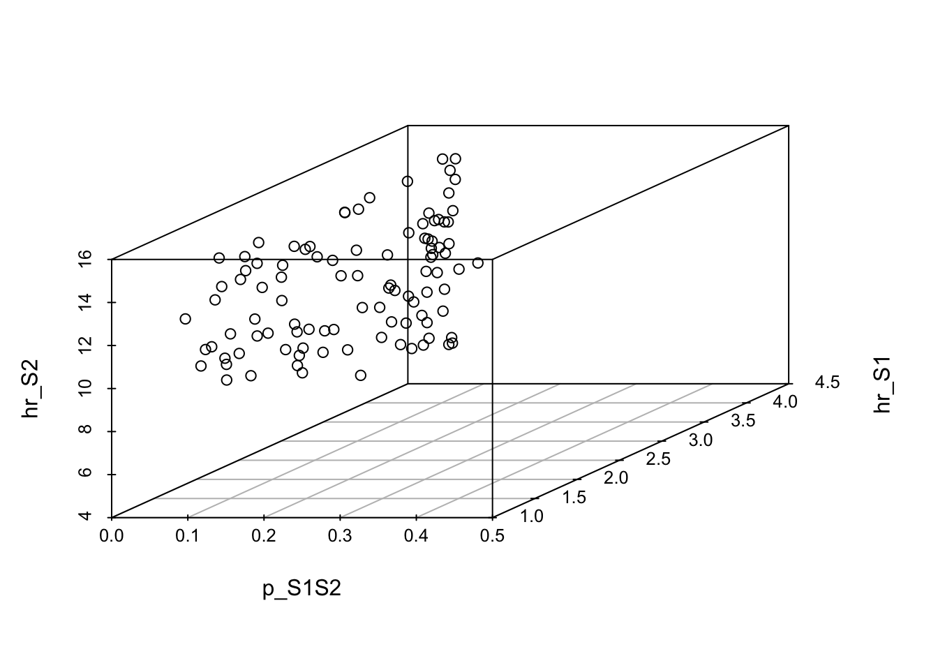
### 07.03 Pairwise plots of top parameter sets  --------------------------------
pairs.panels(m_calib_res[1:100, v_param_names])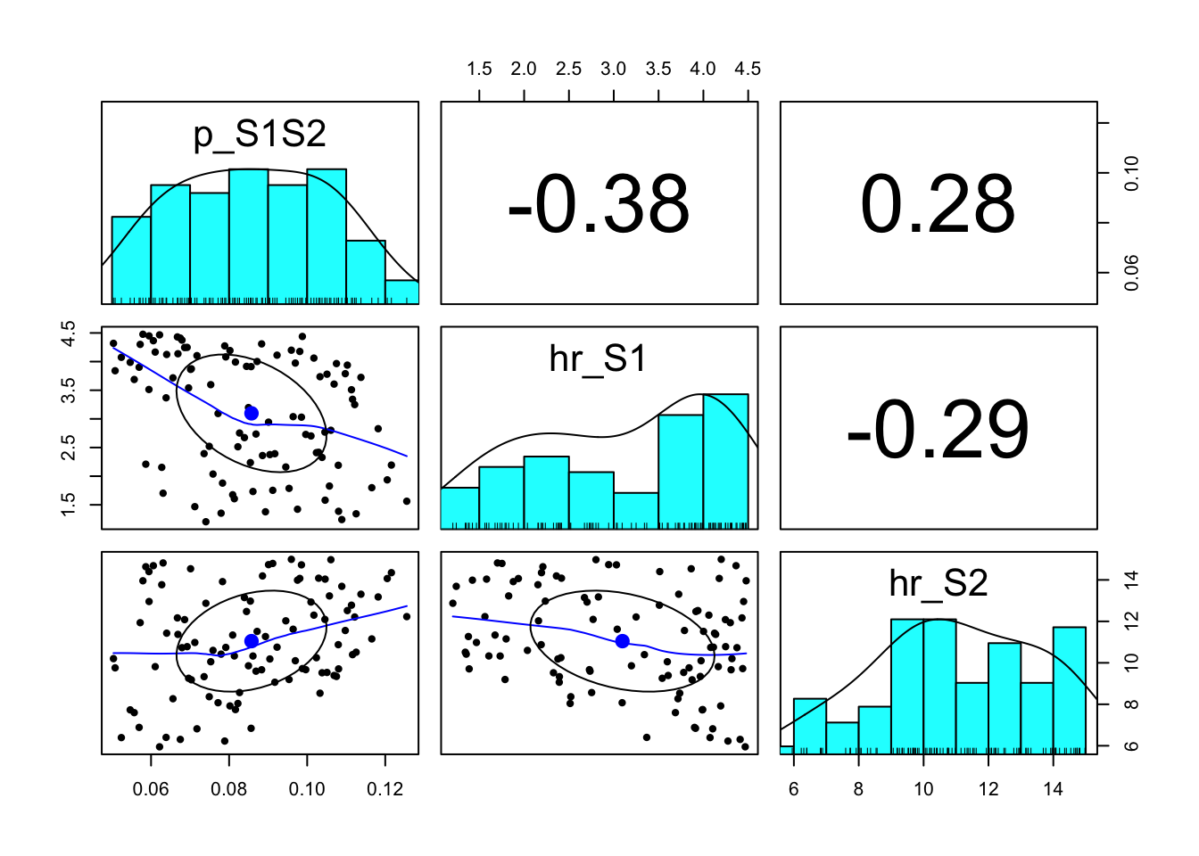
### 07.04 Compare model predictions to targets  --------------------------------
# Compute output from best and worst parameter set
v_out_best  <- run_sick_sicker_markov(m_calib_res[1, ])
v_out_worst <- run_sick_sicker_markov(m_calib_res[n_samp, ])
08 Plot model outputs vs targets (Surv)
# Plot: TARGET 1: Survival ("Surv")
plotrix::plotCI(x = lst_targets$Surv$time, y = lst_targets$Surv$value,
                ui = lst_targets$Surv$ub,
                li = lst_targets$Surv$lb,
                ylim = c(0, 1),
                xlab = "Time", ylab = "Pr Survive")
points(x = lst_targets$Surv$time,
       y = v_out_best$Surv,
       pch = 8, col = "red")
points(x = lst_targets$Surv$time,
       y = v_out_worst$Surv,
       pch = 8, col = "blue")
legend("bottomleft",
       legend = c("Target",
                  "Model-predicted output at best set",
                  "Model-predicted output at worst set"),
       col = c("black", "red", "blue"),
       pch = c(1, 8, 8))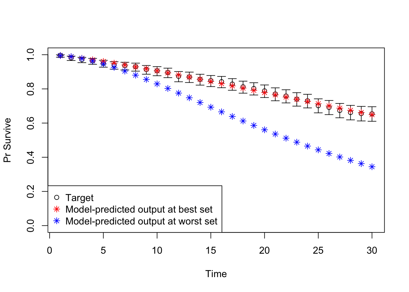
08 Plot model outputs vs targets (Prev)
# Plot: TARGET 2: Prevalence ("Prev")
plotrix::plotCI(x = lst_targets$Prev$time, y = lst_targets$Prev$value,
                ui = lst_targets$Prev$ub,
                li = lst_targets$Prev$lb,
                ylim = c(0, 1),
                xlab = "Time", ylab = "Prev")
points(x = lst_targets$Prev$time,
       y = v_out_best$Prev,
       pch = 8, col = "red")
points(x = lst_targets$Prev$time,
       y = v_out_worst$Prev,
       pch = 8, col = "blue")
legend("topleft",
       legend = c("Target",
                  "Model-predicted output at best set",
                  "Model-predicted output at worst set"),
       col = c("black", "red", "blue"),
       pch = c(1, 8, 8))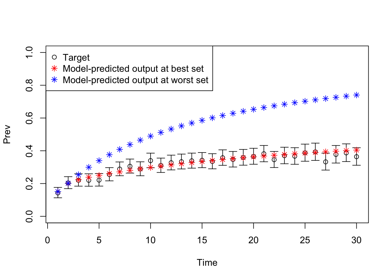
08 Plot model outputs vs targets (PropSick)
# Plot: TARGET 3: PropSick
plotrix::plotCI(x = lst_targets$PropSick$time, y = lst_targets$PropSick$value,
                ui = lst_targets$PropSick$ub,
                li = lst_targets$PropSick$lb,
                ylim = c(0, 1),
                xlab = "Time", ylab = "PropSick")
points(x = lst_targets$PropSick$time,
       y = v_out_best$PropSick,
       pch = 8, col = "red")
points(x = lst_targets$PropSick$time,
       y = v_out_worst$PropSick,
       pch = 8, col = "blue")
legend("topright",
       legend = c("Target",
                  "Model-predicted output at best set",
                  "Model-predicted output at worst set"),
       col = c("black", "red", "blue"),
       pch = c(1, 8, 8))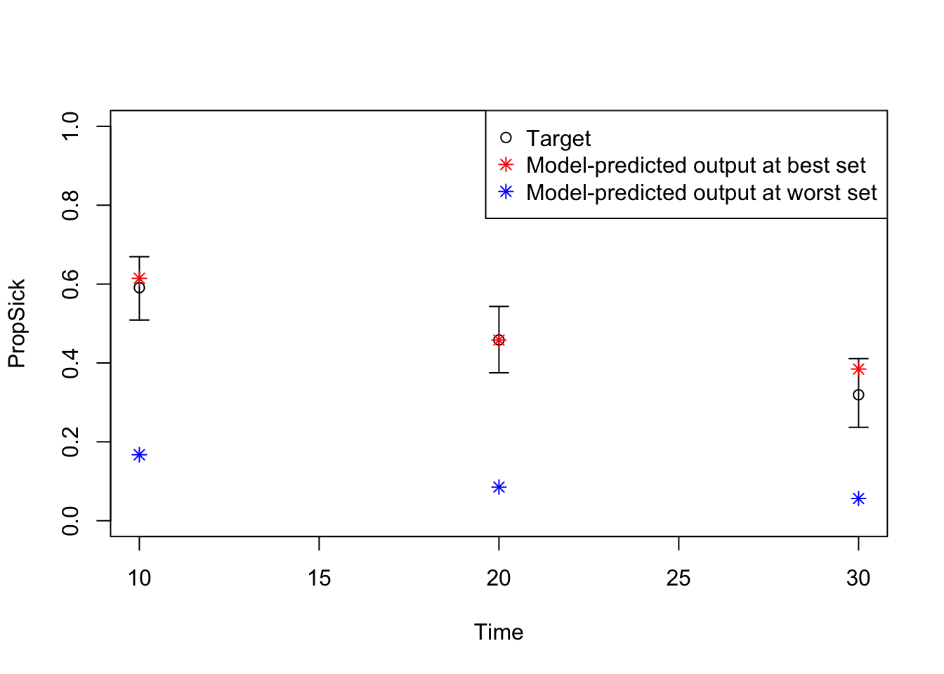
Note: This is a demonstration calibration exercise. In practice, calibration targets would be derived from high-quality epidemiological data, and more sophisticated goodness-of-fit measures might be employed depending on the data structure and modeling objectives.