Sick-Sicker Model: Nelder-Mead Calibration Exercise

01 Calibration Overview

01.01 Model description

The calibration is performed for the Sick-Sicker 4-state cohort Markov model.

[Image of Sick-Sicker Markov model state transition diagram]

Inputs to be calibrated: - p_S1S2 - hr_S1 - hr_S2

Targets: - Surv - Prev - PropSick

01.02 Calibration method

• Search method: Nelder-Mead algorithm
• Goodness-of-fit measure: Sum of Log-Likelihood

02 Setup

# ******************************************************************************
# 02 Setup ---------------------------------------------------------------------
# ******************************************************************************

### 02.01 Clear environment ---------------------------------------------------
rm(list = ls())

### 02.02 Load packages -------------------------------------------------------
# Install pacman if not present
if (!requireNamespace("pacman", quietly = TRUE)) install.packages("pacman")

# Load pacman
library(pacman)

# Load (install if needed) CRAN packages
p_load(
  lhs,           # Latin Hypercube Sampling
  plotrix,       # Plotting with confidence intervals
  psych,         # Pairs panels
  scatterplot3d, # 3D scatter plots
  ggplot2,       # Advanced plotting
  GGally,        # Pairwise plots
  mvtnorm,       # Multivariate normal distribution
  matrixcalc,    # To evaluate if matrix is positive definite
  Matrix         # To compute nearest positive definite matrix
)

The downloaded binary packages are in
    /var/folders/7d/cm50s82x4_z_xmhpt0hc5ddh0000gp/T//RtmpjxZRsk/downloaded_packages

03 Load calibration targets

# ******************************************************************************
# 03 Load calibration targets --------------------------------------------------
# ******************************************************************************

### 03.01 Load target data ----------------------------------------------------
load("data/SickSicker_CalibTargets.RData")
lst_targets <- SickSicker_targets

### 03.02 Visualize calibration targets ---------------------------------------
# TARGET 1: Survival ("Surv")
plotrix::plotCI(x = lst_targets$Surv$time, 
                y = lst_targets$Surv$value, 
                ui = lst_targets$Surv$ub,
                li = lst_targets$Surv$lb,
                ylim = c(0, 1), 
                xlab = "Time", 
                ylab = "Pr Survive")

# TARGET 2: Prevalence ("Prev")
plotrix::plotCI(x = lst_targets$Prev$time, 
                y = lst_targets$Prev$value,
                ui = lst_targets$Prev$ub,
                li = lst_targets$Prev$lb,
                ylim = c(0, 1),
                xlab = "Time", 
                ylab = "Prev")

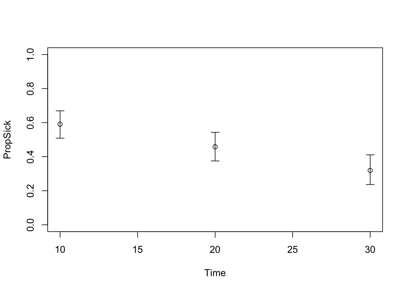
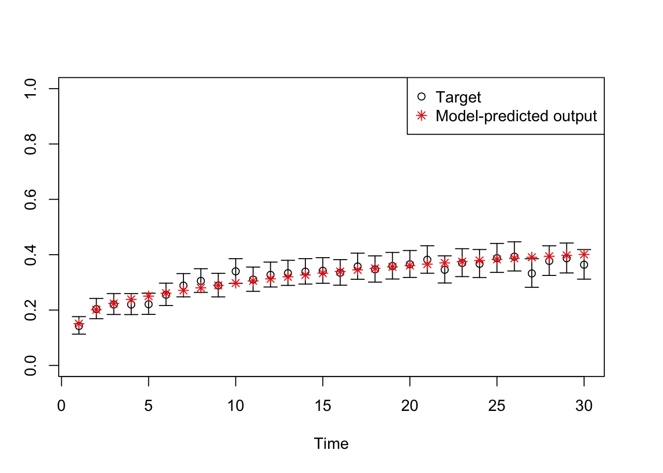
# TARGET 3: Proportion who are Sick ("PropSick"), among all those afflicted (Sick+Sicker)
plotrix::plotCI(x = lst_targets$PropSick$time, 
                y = lst_targets$PropSick$value,
                ui = lst_targets$PropSick$ub,
                li = lst_targets$PropSick$lb,
                ylim = c(0, 1),
                xlab = "Time", 
                ylab = "PropSick")

04 Load model as a function

# ******************************************************************************
# 04 Load model as a function --------------------------------------------------
# ******************************************************************************

### 04.01 Source model function -----------------------------------------------
# Function inputs: parameters to be estimated through calibration
# Function outputs: model predictions corresponding to target data
source("code/functions/SickSicker_MarkovModel_Function.R") # creates run_sick_sicker_markov()

### 04.02 Test model function -------------------------------------------------
v_params_test <- c(p_S1S2 = 0.105, hr_S1 = 3, hr_S2 = 10)
run_sick_sicker_markov(v_params_test) # Test: function works correctly

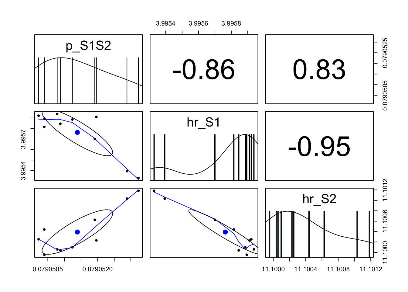
$Surv
        1         2         3         4         5         6         7         8 
0.9950000 0.9885362 0.9810784 0.9728008 0.9637994 0.9541472 0.9439082 0.9331413 
        9        10        11        12        13        14        15        16 
0.9219015 0.9102402 0.8982055 0.8858421 0.8731922 0.8602948 0.8471865 0.8339014 
       17        18        19        20        21        22        23        24 
0.8204713 0.8069256 0.7932918 0.7795955 0.7658602 0.7521079 0.7383588 0.7246318 
       25        26        27        28        29        30 
0.7109441 0.6973115 0.6837488 0.6702694 0.6568856 0.6436086 

$Prev
        1         2         3         4         5         6         7         8 
0.1507538 0.2018249 0.2267624 0.2443252 0.2593508 0.2731265 0.2860289 0.2981972 
        9        10        11        12        13        14        15        16 
0.3097057 0.3206084 0.3309506 0.3407725 0.3501104 0.3589973 0.3674630 0.3755352 
       17        18        19        20        21        22        23        24 
0.3832387 0.3905968 0.3976304 0.4043591 0.4108009 0.4169723 0.4228887 0.4285642 
       25        26        27        28        29        30 
0.4340120 0.4392445 0.4442729 0.4491079 0.4537594 0.4582367 

$PropSick
       10        20        30 
0.5372139 0.3734392 0.2997246 

05 Calibration specifications

# ******************************************************************************
# 05 Calibration specifications ------------------------------------------------
# ******************************************************************************

### 05.01 Set random seed -----------------------------------------------------
set.seed(072218) # For reproducible sequence of random numbers

### 05.02 Define calibration parameters ---------------------------------------
# Number of initial starting points
n_init <- 100

# Names and number of parameters to calibrate
v_param_names <- c("p_S1S2", "hr_S1", "hr_S2")
n_param       <- length(v_param_names)

# Search space bounds
lb <- c(p_S1S2 = 0.01, hr_S1 = 1.0, hr_S2 = 5)  # lower bound
ub <- c(p_S1S2 = 0.50, hr_S1 = 4.5, hr_S2 = 15) # upper bound

### 05.03 Define calibration targets ------------------------------------------
v_target_names <- c("Surv", "Prev", "PropSick")
n_target       <- length(v_target_names)

06 Goodness-of-fit function

# ******************************************************************************
# 06 Goodness-of-fit function --------------------------------------------------
# ******************************************************************************

### 06.01 Function to calculate goodness-of-fit -------------------------------
f_gof <- function(v_params){
  
  # Run model for parameter set v_params
  model_res <- run_sick_sicker_markov(v_params)
  
  # Calculate goodness-of-fit of model outputs to targets
  v_GOF <- numeric(n_target)
  
  # TARGET 1: Survival ("Surv") - log likelihood  
  v_GOF[1] <- sum(dnorm(x = lst_targets$Surv$value,
                        mean = model_res$Surv,
                        sd = lst_targets$Surv$se,
                        log = TRUE))
  
  # TARGET 2: Prevalence ("Prev") - log likelihood
  v_GOF[2] <- sum(dnorm(x = lst_targets$Prev$value,
                        mean = model_res$Prev,
                        sd = lst_targets$Prev$se,
                        log = TRUE))
  
  # TARGET 3: Proportion Sick ("PropSick") - log likelihood
  v_GOF[3] <- sum(dnorm(x = lst_targets$PropSick$value,
                        mean = model_res$PropSick,
                        sd = lst_targets$PropSick$se,
                        log = TRUE))
  
  # OVERALL - weighted sum (can give different targets different weights)
  v_weights <- rep(1, n_target)
  GOF_overall <- sum(v_GOF[1:n_target] * v_weights)
  
  return(GOF_overall)
}

### 06.02 Test goodness-of-fit function ---------------------------------------
f_gof(v_params = v_params_test)

[1] 135.7134

07 Run calibration using Nelder-Mead

# ******************************************************************************
# 07 Run calibration using Nelder-Mead -----------------------------------------
# ******************************************************************************

### 07.01 Record start time ---------------------------------------------------
t_init <- Sys.time()

### 07.02 Sample initial starting values --------------------------------------
v_params_init <- matrix(nrow = n_init, ncol = n_param)
for (i in 1:n_param) {
  v_params_init[, i] <- runif(n_init, min = lb[i], max = ub[i])
}
colnames(v_params_init) <- v_param_names

### 07.03 Initialize results storage ------------------------------------------
m_calib_res <- matrix(nrow = n_init, ncol = n_param + 1, 
                      dimnames = list(paste0("par_id_", 1:n_init),
                                      c(v_param_names, "Overall_fit")))
l_fit_nm <- vector(mode = "list", length = n_init)
names(l_fit_nm) <- paste0("par_id_", 1:n_init)

### 07.04 Run Nelder-Mead for each starting point -----------------------------
for (j in 1:n_init) {
  
  # Use optim() with Nelder-Mead algorithm
  l_fit_nm[[j]] <- optim(v_params_init[j, ], f_gof,
                         control = list(fnscale = -1, # switches from minimization to maximization
                                        maxit = 1000), 
                         hessian = TRUE)
  m_calib_res[j, ] <- c(l_fit_nm[[j]]$par, l_fit_nm[[j]]$value)
  
  ### to use a simulated annealing instead ###
  # fit_sa <- optim(v_params_init[j,], f_gof,
  #                 method = c("SANN"),  # switches to using simulated annealing
  #                 control = list(temp = 10, tmax = 10, # algorithm tuning parameters
  #                                fnscale = -1, maxit = 1000),
  #                 hessian = T)
  # m_calib_res[j,] = c(fit_sa$par,fit_sa$value)
  
  ### to use a genetic algorithm instead ###
  # library(DEoptim)
  # f_fitness <- function(params){
  #   names(params) = v_param_names
  #   return(-f_gof(params))}
  # fit_ga = DEoptim(f_fitness, lower=lb, upper=ub)
  # m_calib_res[j,] = c(fit_ga$optim$bestmem,-1*fit_ga$optim$bestval)
  
}

### 07.05 Calculate computation time ------------------------------------------
comp_time <- Sys.time() - t_init
comp_time

Time difference of 2.251042 secs

08 Explore calibration results

# ******************************************************************************
# 08 Explore calibration results -----------------------------------------------
# ******************************************************************************

### 08.01 Identify best-fitting parameter sets --------------------------------
# Arrange parameter sets in order of fit
m_calib_res <- m_calib_res[order(-m_calib_res[, "Overall_fit"]), ]

# Best parameter set
v_param_best <- m_calib_res[1, -4]
v_param_best

     p_S1S2       hr_S1       hr_S2 
 0.07905191  3.99569989 11.10062670 

# Obtain id for best set
id_best_set <- rownames(m_calib_res)[1]

# Examine the top 10 best-fitting sets
m_calib_res[1:10, ]

              p_S1S2    hr_S1    hr_S2 Overall_fit
par_id_88 0.07905191 3.995700 11.10063    176.8825
par_id_51 0.07905022 3.995922 11.10025    176.8825
par_id_48 0.07905039 3.995815 11.10044    176.8825
par_id_61 0.07905078 3.995938 11.10006    176.8825
par_id_79 0.07905124 3.995886 11.10010    176.8825
par_id_15 0.07905288 3.995394 11.10103    176.8825
par_id_10 0.07905323 3.995329 11.10118    176.8825
par_id_91 0.07905088 3.995845 11.10004    176.8825
par_id_21 0.07905196 3.995910 11.10023    176.8825
par_id_49 0.07905040 3.995894 11.09995    176.8825

### 08.02 Visualize best-fitting parameter sets in 3D -------------------------
scatterplot3d(x = m_calib_res[1:10, 1],
              y = m_calib_res[1:10, 2],
              z = m_calib_res[1:10, 3],
              xlim = c(lb[1], ub[1]), 
              ylim = c(lb[2], ub[2]), 
              zlim = c(lb[3], ub[3]),
              xlab = v_param_names[1], 
              ylab = v_param_names[2], 
              zlab = v_param_names[3])

### 08.03 Pairwise plots of top parameter sets --------------------------------
pairs.panels(m_calib_res[1:10, v_param_names])

### 08.04 Compare model predictions to targets --------------------------------
# Compute output from best parameter set
v_out_best <- run_sick_sicker_markov(m_calib_res[1, ])

# Plot: TARGET 1: Survival
plotrix::plotCI(x = lst_targets$Surv$time, 
                y = lst_targets$Surv$value, 
                ui = lst_targets$Surv$ub,
                li = lst_targets$Surv$lb,
                ylim = c(0, 1), 
                xlab = "Time", 
                ylab = "Pr Survive")

points(x = lst_targets$Surv$time, 
       y = v_out_best$Surv, 
       pch = 8, col = "red")

legend("bottomleft", 
       legend = c("Target", "Model-predicted output"),
       col = c("black", "red"), 
       pch = c(1, 8))

# Plot: TARGET 2: Prevalence
plotrix::plotCI(x = lst_targets$Prev$time, 
                y = lst_targets$Prev$value,
                ui = lst_targets$Prev$ub,
                li = lst_targets$Prev$lb,
                ylim = c(0, 1),
                xlab = "Time", 
                ylab = "Prev")

points(x = lst_targets$Prev$time,
       y = v_out_best$Prev,
       pch = 8, col = "red")

legend("topright",
       legend = c("Target", "Model-predicted output"),
       col = c("black", "red"), 
       pch = c(1, 8))

# Plot: TARGET 3: PropSick
plotrix::plotCI(x = lst_targets$PropSick$time, 
                y = lst_targets$PropSick$value,
                ui = lst_targets$PropSick$ub,
                li = lst_targets$PropSick$lb,
                ylim = c(0, 1),
                xlab = "Time", 
                ylab = "PropSick")

points(x = lst_targets$PropSick$time,
       y = v_out_best$PropSick,
       pch = 8, col = "red")

legend("topright",
       legend = c("Target", "Model-predicted output"),
       col = c("black", "red"), 
       pch = c(1, 8))

09 Uncertainty quantification

# ******************************************************************************
# 09 Uncertainty quantification ------------------------------------------------
# ******************************************************************************

### 09.01 Extract Hessian matrix ----------------------------------------------
m_hess <- l_fit_nm[[id_best_set]]$hessian
m_hess

              p_S1S2       hr_S1     hr_S2
p_S1S2 -136767.08465 -611.443763 27.989386
hr_S1     -611.44376  -11.528516 -4.893202
hr_S2       27.98939   -4.893202 -3.431245

# check if hessian is negative definite
eigen(m_hess)$values

[1] -4.188857e-01 -1.180140e+01 -1.367698e+05

### 09.02 Covariance matrix ---------------------------------------------------
# Check if HESSIAN is Positive Definite; If not, make covariance 
# Positive Definite
# Is Positive Definite?
if (!is.positive.definite(-m_hess)) {
  print("Hessian is NOT Positive Definite")
  m_cov <- solve(-m_hess)
  print("Compute nearest positive definite matrix for COV matrix using `nearPD` function")
  m_cov <- Matrix::nearPD(m_cov)$mat
} else{
  print("Hessian IS Positive Definite")
  print("No additional adjustment to COV matrix")
  m_cov <- solve(-m_hess)
}

[1] "Hessian IS Positive Definite"
[1] "No additional adjustment to COV matrix"

### 09.03 Correlation matrix ---------------------------------------------------
m_cor <- cov2cor(m_cov)
m_cor

           p_S1S2      hr_S1      hr_S2
p_S1S2  1.0000000 -0.8263510  0.7648383
hr_S1  -0.8263510  1.0000000 -0.9142818
hr_S2   0.7648383 -0.9142818  1.0000000

### 09.04 Calculate standard errors -------------------------------------------
m_se <- sqrt(diag(m_cov))
m_se

     p_S1S2       hr_S1       hr_S2 
0.004805558 0.832423192 1.333820741 

### 09.05 Calculate 95% confidence interval -----------------------------------
m_confint <- cbind(v_param_best - 1.96*m_se,
                   v_param_best + 1.96*m_se)
colnames(m_confint) <- c("LB", "UB")
m_confint

               LB          UB
p_S1S2 0.06963302  0.08847081
hr_S1  2.36415044  5.62724935
hr_S2  8.48633805 13.71491535

### 09.06 Sample from multivariate normal distribution ------------------------
n_samp <- 1000
m_param_best_sample <- rmvnorm(n = n_samp, 
                               mean = v_param_best, 
                               sigma = m_cov)
colnames(m_param_best_sample) <- v_param_names

### 09.07 Visualize parameter samples -----------------------------------------
pairs.panels(m_param_best_sample)

### 09.08 Advanced visualization: pairwise correlations -----------------------
gg_nm_pairs_corr <- GGally::ggpairs(
  data.frame(m_param_best_sample),
  upper = list(continuous = wrap("cor",
                                 color = "black",
                                 size = 5)),
  diag = list(continuous = wrap("barDiag",
                                alpha = 0.8)),
  lower = list(continuous = wrap("points", 
                                 alpha = 0.3,
                                 size = 0.7)),
  columnLabels = v_param_names
) +
  theme_bw(base_size = 18) +
  theme(axis.title.x = element_blank(),
        axis.text.x  = element_text(size = 14),
        axis.title.y = element_blank(),
        axis.text.y  = element_blank(),
        axis.ticks.y = element_blank(),
        strip.background = element_rect(fill = "white",
                                        color = "white"),
        strip.text = element_text(hjust = 0))
gg_nm_pairs_corr

`stat_bin()` using `bins = 30`. Pick better value `binwidth`.
`stat_bin()` using `bins = 30`. Pick better value `binwidth`.
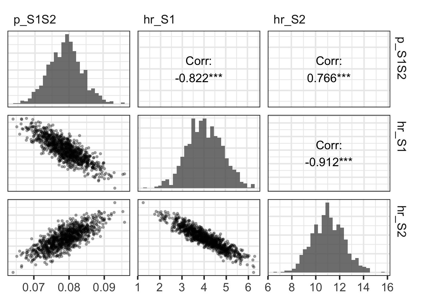
`stat_bin()` using `bins = 30`. Pick better value `binwidth`.

---

Note: This exercise demonstrates calibration using the Nelder-Mead algorithm via the optim() function in R. This method is a local search algorithm and depends on the initial values provided.