### 03.01 Load target data  ----------------------------------------------------
load("data/SickSicker_CalibTargets.RData")
lst_targets <- SickSicker_targetsSick-Sicker Model: Incremental Mixture Importance Sampling (IMIS) Exercise
01 Calibration Overview
01.01 Model Description
The calibration is performed for the Sick-Sicker 4-state cohort Markov model, which represents the natural history of a chronic disease.
The model includes four health states:
- Healthy (H)
- Sick (S1)
- Sicker (S2)
- Dead (D)
The following model parameters are calibrated:
p_S1S2: Probability of progression from Sick (S1) to Sicker (S2)
hr_S1: Mortality hazard ratio in the Sick state relative to Healthy
hr_S2: Mortality hazard ratio in the Sicker state relative to Healthy
Calibration targets include:
- Survival (
Surv): Proportion of the cohort alive over time
- Prevalence (
Prev): Proportion of the cohort with disease (Sick + Sicker)
- Proportion Sick (
PropSick): Among diseased individuals, the proportion in the Sick (S1) state
01.02 Calibration method
- Search method: Incremental Mixture Importance Sampling (IMIS)
- Goodness-of-fit measure: Sum of Log-Likelihood
02 Setup
03 Load calibration targets
TARGET 1: Survival (“Surv”)
plotrix::plotCI(x = lst_targets$Surv$time, y = lst_targets$Surv$value,
                ui = lst_targets$Surv$ub,
                li = lst_targets$Surv$lb,
                ylim = c(0, 1),
                xlab = "Time", ylab = "Pr Survive")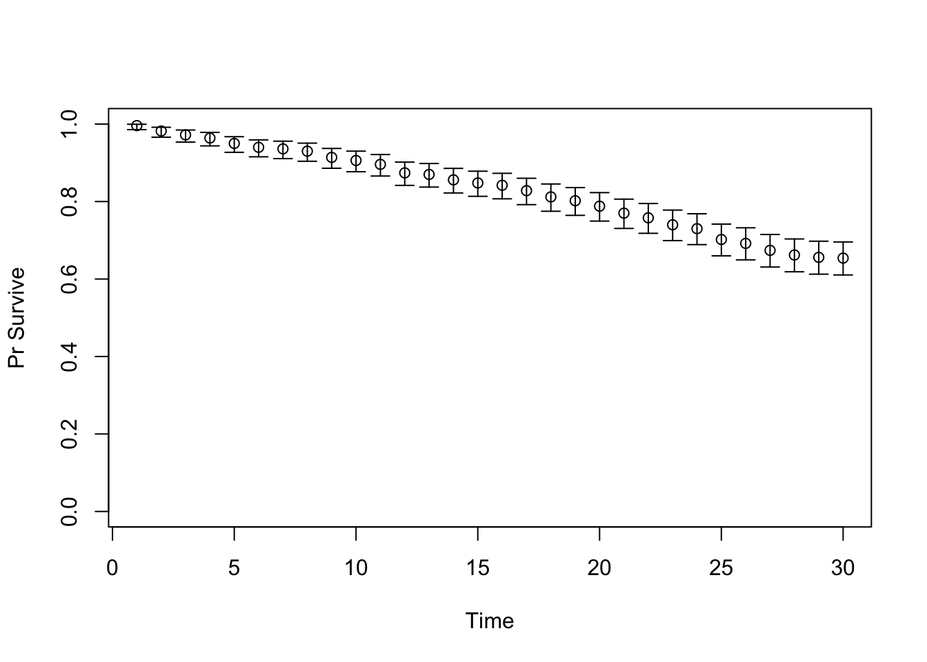
TARGET 2: Prevalence (“Prev”)
plotrix::plotCI(x = lst_targets$Prev$time, y = lst_targets$Prev$value,
                ui = lst_targets$Prev$ub,
                li = lst_targets$Prev$lb,
                ylim = c(0, 1),
                xlab = "Time", ylab = "Prev")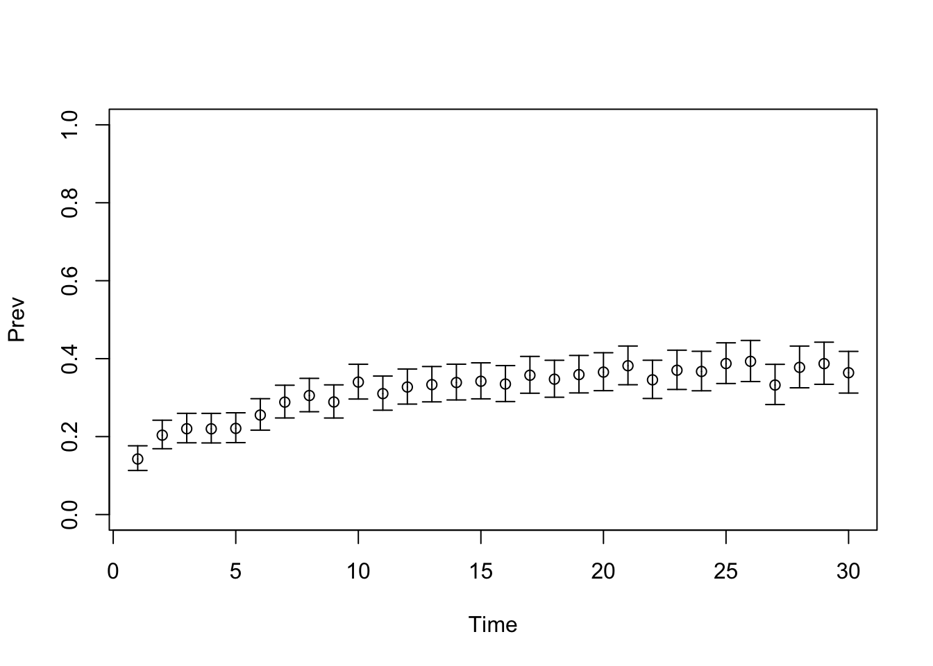
TARGET 3: Proportion who are Sick (“PropSick”), among all those afflicted (Sick+Sicker)
plotrix::plotCI(x = lst_targets$PropSick$time, y = lst_targets$PropSick$value,
                ui = lst_targets$PropSick$ub,
                li = lst_targets$PropSick$lb,
                ylim = c(0, 1),
                xlab = "Time", ylab = "PropSick")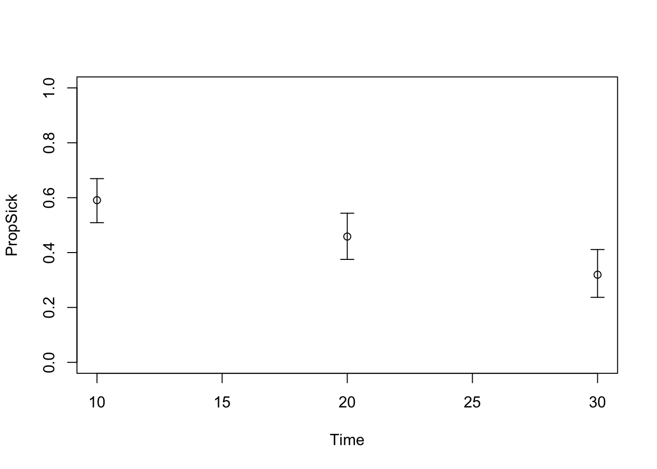
04 Load model as a function
### 04.01 Source model function  -----------------------------------------------
# Function inputs: parameters to be estimated through calibration
# Function outputs: model predictions corresponding to target data
source("code/Functions/SickSicker_MarkovModel_Function.R") # creates the function run_sick_sicker_markov()

### 04.02 Test model function  -------------------------------------------------
v_params_test <- c(p_S1S2 = 0.105, hr_S1 = 3, hr_S2 = 10)
run_sick_sicker_markov(v_params_test) # Test: function works correctly
$Surv
1 2 3 4 5 6 7 8
0.9950000 0.9885362 0.9810784 0.9728008 0.9637994 0.9541472 0.9439082 0.9331413
9 10 11 12 13 14 15 16
0.9219015 0.9102402 0.8982055 0.8858421 0.8731922 0.8602948 0.8471865 0.8339014
17 18 19 20 21 22 23 24
0.8204713 0.8069256 0.7932918 0.7795955 0.7658602 0.7521079 0.7383588 0.7246318
25 26 27 28 29 30
0.7109441 0.6973115 0.6837488 0.6702694 0.6568856 0.6436086
$Prev
1 2 3 4 5 6 7 8
0.1507538 0.2018249 0.2267624 0.2443252 0.2593508 0.2731265 0.2860289 0.2981972
9 10 11 12 13 14 15 16
0.3097057 0.3206084 0.3309506 0.3407725 0.3501104 0.3589973 0.3674630 0.3755352
17 18 19 20 21 22 23 24
0.3832387 0.3905968 0.3976304 0.4043591 0.4108009 0.4169723 0.4228887 0.4285642
25 26 27 28 29 30
0.4340120 0.4392445 0.4442729 0.4491079 0.4537594 0.4582367
$PropSick
10 20 30
0.5372139 0.3734392 0.2997246 05 Calibration specifications
### 05.01 Set random seed  -----------------------------------------------------
set.seed(072218) # For reproducible sequence of random numbers

### 05.02 Define calibration parameters  ---------------------------------------
# Number of posterior samples desired
n_resamp <- 1000

# Names and number of parameters to calibrate
v_param_names <- c("p_S1S2", "hr_S1", "hr_S2")
n_param       <- length(v_param_names)

# Search space bounds
v_lb <- c(p_S1S2 = 0.01, hr_S1 = 1, hr_S2 = 1)    # lower bound
v_ub <- c(p_S1S2 = 0.50, hr_S1 = 12, hr_S2 = 25)  # upper bound

### 05.03 Define calibration targets  ------------------------------------------
v_target_names <- c("Surv", "Prev", "PropSick")
n_target       <- length(v_target_names)

### 05.04 Define target indices  -----------------------------------------------
# A list to index each target
l_index <- list(
  Surv     = 1:30,  # 30 time points
  Prev     = 1:30,  # 30 time points
  PropSick = 3      # 3 time points
)
06 Prior distribution functions
### 06.01 Function to sample from prior  ---------------------------------------
sample_prior <- function(n_samp){
  # Generate Latin Hypercube Sample
  m_lhs_unit   <- randomLHS(n = n_samp, k = n_param)
  m_param_samp <- matrix(nrow = n_samp, ncol = n_param)
  colnames(m_param_samp) <- v_param_names

  # Transform to parameter space using uniform distribution
  for (i in 1:n_param) {
    m_param_samp[, i] <- qunif(m_lhs_unit[, i],
                               min = v_lb[i],
                               max = v_ub[i])
  }
  return(m_param_samp)
}

### 06.02 Visualize prior samples  ---------------------------------------------
pairs.panels(sample_prior(1000))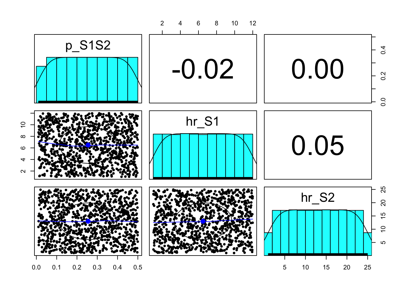
### 06.03 Function to calculate log-prior  -------------------------------------
calc_log_prior <- function(v_params){
  if (is.null(dim(v_params))) { # If vector, change to matrix
    v_params <- t(v_params)
  }
  n_samp <- nrow(v_params)
  colnames(v_params) <- v_param_names
  lprior <- rep(0, n_samp)

  # Calculate log-prior using uniform distribution
  for (i in 1:n_param) {
    lprior <- lprior + dunif(v_params[, i],
                             min = v_lb[i],
                             max = v_ub[i],
                             log = TRUE)
  }
  return(lprior)
}

### 06.04 Function to calculate prior  -----------------------------------------
calc_prior <- function(v_params) {
  exp(calc_log_prior(v_params))
}

### 06.05 Test prior functions  ------------------------------------------------
calc_log_prior(v_params = v_params_test)
p_S1S2
-4.862599 calc_log_prior(v_params = sample_prior(10)) [1] -4.862599 -4.862599 -4.862599 -4.862599 -4.862599 -4.862599 -4.862599
[8] -4.862599 -4.862599 -4.862599calc_prior(v_params = v_params_test) p_S1S2
0.007730365 calc_prior(v_params = sample_prior(10)) [1] 0.007730365 0.007730365 0.007730365 0.007730365 0.007730365 0.007730365
[7] 0.007730365 0.007730365 0.007730365 0.00773036507 Likelihood functions
### 07.01 Function to calculate log-likelihood  --------------------------------
calc_log_lik <- function(v_params){
  if (is.null(dim(v_params))) { # If vector, change to matrix
    v_params <- t(v_params)
  }
  n_samp <- nrow(v_params)
  v_llik <- matrix(0, nrow = n_samp, ncol = n_target)
  llik_overall <- numeric(n_samp)

  for (j in 1:n_samp) { # j = 1
    jj <- tryCatch({
      # Run model for parameter set v_params
      model_res <- run_sick_sicker_markov(v_params[j, ])

      # Calculate log-likelihood for TARGET 1: Survival
      v_llik[j, 1] <- sum(dnorm(x = lst_targets$Surv$value[l_index$Surv],
                                mean = model_res$Surv[l_index$Surv],
                                sd = lst_targets$Surv$se[l_index$Surv],
                                log = TRUE))

      # Calculate log-likelihood for TARGET 2: Prevalence
      v_llik[j, 2] <- sum(dnorm(x = lst_targets$Prev$value[l_index$Prev],
                                mean = model_res$Prev[l_index$Prev],
                                sd = lst_targets$Prev$se[l_index$Prev],
                                log = TRUE))

      # Calculate log-likelihood for TARGET 3: PropSick
      v_llik[j, 3] <- sum(dnorm(x = lst_targets$PropSick$value[l_index$PropSick],
                                mean = model_res$PropSick[l_index$PropSick],
                                sd = lst_targets$PropSick$se[l_index$PropSick],
                                log = TRUE))

      # Calculate overall log-likelihood
      llik_overall[j] <- sum(v_llik[j, ])
    }, error = function(e) NA)

    if (is.na(jj)) { llik_overall[j] <- -Inf }
  }
  return(llik_overall)
}

### 07.02 Function to calculate likelihood  ------------------------------------
calc_likelihood <- function(v_params){
  exp(calc_log_lik(v_params))
}

### 07.03 Test likelihood functions  -------------------------------------------
calc_log_lik(v_params = v_params_test)
[1] 134.1498calc_log_lik(v_params = sample_prior(10)) [1] -1646.99811 10.79923 -503.66998 -323.45784 -1030.04215 -2138.32715
[7] -1054.98821 113.89390 -3091.94792 -3249.87925calc_likelihood(v_params = v_params_test)[1] 1.821927e+58calc_likelihood(v_params = sample_prior(10)) [1] 0.000000e+00 0.000000e+00 3.504052e-34 9.209882e+39 1.601446e-83
[6] 0.000000e+00 0.000000e+00 0.000000e+00 0.000000e+00 0.000000e+0008 Posterior distribution functions
### 08.01 Function to calculate log-posterior  ---------------------------------
calc_log_post <- function(v_params) {
  lpost <- calc_log_prior(v_params) + calc_log_lik(v_params)
  return(lpost)
}

### 08.02 Function to calculate posterior  -------------------------------------
calc_post <- function(v_params) {
  exp(calc_log_post(v_params))
}

### 08.03 Test posterior functions  --------------------------------------------
calc_log_post(v_params = v_params_test)
p_S1S2
129.2872 calc_log_post(v_params = sample_prior(10)) [1] -843.93691 -2350.29509 20.77087 -67.73469 -685.35122 47.02586
[7] -2176.82881 -2921.51322 -2212.58392 -2357.23784calc_post(v_params = v_params_test) p_S1S2
1.408416e+56 calc_post(v_params = sample_prior(10)) [1] 7.774168e+05 0.000000e+00 9.704347e-126 0.000000e+00 1.444577e-221
[6] 3.361193e+64 0.000000e+00 0.000000e+00 0.000000e+00 1.065450e-24509 Run Bayesian calibration using IMIS
### 09.01 Record start time  ---------------------------------------------------
t_init <- Sys.time()

### 09.02 Define IMIS functions  -----------------------------------------------
prior        <- calc_prior
likelihood   <- calc_likelihood
sample.prior <- sample_prior

### 09.03 Run IMIS algorithm  --------------------------------------------------
fit_imis <- IMIS(
  B = 1000,         # Incremental sample size at each iteration
  B.re = n_resamp,  # Desired posterior sample size
  number_k = 10,    # Maximum number of iterations
  D = 0             # Number of samples to be deleted at each iteration
)
[1] "10000 likelihoods are evaluated in 0.02 minutes"
[1] "Stage MargLike UniquePoint MaxWeight ESS"
[1] 1.000 163.845 24.203 0.527 3.097
[1] 2.000 163.756 178.561 0.025 95.420
[1] 3.000 163.819 476.562 0.005 497.194
[1] 4.000 163.815 557.695 0.003 662.780
[1] 5.000 163.791 648.784 0.002 945.967### 09.04 Extract posterior samples -------------------------------------------
m_calib_res <- fit_imis$resample
### 09.05 Calculate posterior diagnostics -------------------------------------
# Calculate log-likelihood and posterior probability for each sample
m_calib_res <- cbind(
m_calib_res,
"Overall_fit" = calc_log_lik(m_calib_res[, v_param_names]),
"Posterior_prob" = calc_post(m_calib_res[, v_param_names])
)
# Normalize posterior probabilities
m_calib_res[, "Posterior_prob"] <- m_calib_res[, "Posterior_prob"] /
sum(m_calib_res[, "Posterior_prob"])
### 09.06 Calculate computation time ------------------------------------------
comp_time <- Sys.time() - t_init
comp_timeTime difference of 1.945518 secs10 Explore posterior distribution
### 10.01 Visualize posterior samples in 3D  -----------------------------------
# Color points by posterior probability
v_post_color <- scales::rescale(m_calib_res[, "Posterior_prob"])

s3d <- scatterplot3d(
  x = m_calib_res[, 1],
  y = m_calib_res[, 2],
  z = m_calib_res[, 3],
  color = scales::alpha("black", v_post_color),
  xlim = c(v_lb[1], v_ub[1]),
  ylim = c(v_lb[2], v_ub[2]),
  zlim = c(v_lb[3], v_ub[3]),
  xlab = v_param_names[1],
  ylab = v_param_names[2],
  zlab = v_param_names[3]
)

# Add centers of Gaussian components
s3d$points3d(fit_imis$center, col = "red", pch = 8)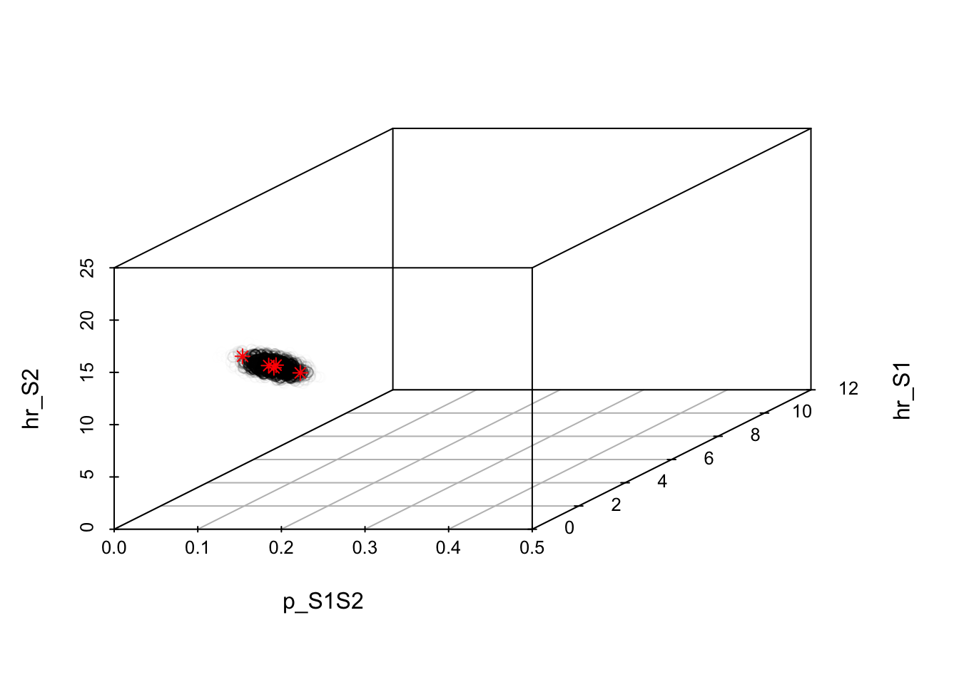
### 10.02 Pairwise plots with marginal histograms  -----------------------------
pairs.panels(m_calib_res[, v_param_names])
### 10.03 Calculate posterior summary statistics  ------------------------------
# Posterior mean
v_calib_post_mean <- colMeans(m_calib_res[, v_param_names])
v_calib_post_mean
p_S1S2 hr_S1 hr_S2
0.07822368 4.05205376 11.07280295 # Posterior median and 95% credible interval
m_calib_res_95cr <- colQuantiles(m_calib_res[, v_param_names],
probs = c(0.025, 0.5, 0.975))
m_calib_res_95cr 2.5% 50% 97.5%
p_S1S2 0.06803991 0.07814902 0.08902665
hr_S1 2.31892327 4.07432464 5.66988301
hr_S2 8.55722643 11.08868123 13.80817681# Maximum-a-posteriori (MAP) parameter set
v_calib_map <- m_calib_res[which.max(m_calib_res[, "Posterior_prob"]), ]
### 10.04 Compare model predictions to targets --------------------------------
# Compute output from MAP
v_out_map <- run_sick_sicker_markov(v_calib_map[v_param_names])
# Compute output from posterior mean
v_out_post_mean <- run_sick_sicker_markov(v_calib_post_mean)11 Plot model outputs vs targets (Surv)
# Plot: TARGET 1: Survival
plotrix::plotCI(x = lst_targets$Surv$time,
                y = lst_targets$Surv$value,
                ui = lst_targets$Surv$ub,
                li = lst_targets$Surv$lb,
                ylim = c(0, 1),
                xlab = "Time",
                ylab = "Pr Survive")

points(x = lst_targets$Surv$time,
       y = v_out_map$Surv,
       pch = 8, col = "red")

points(x = lst_targets$Surv$time,
       y = v_out_post_mean$Surv,
       pch = 2, col = "blue")

legend("bottomleft",
       legend = c("Target",
                  "Model-predicted output using MAP",
                  "Model-predicted output using posterior mean"),
       col = c("black", "red", "blue"),
       pch = c(1, 8, 2))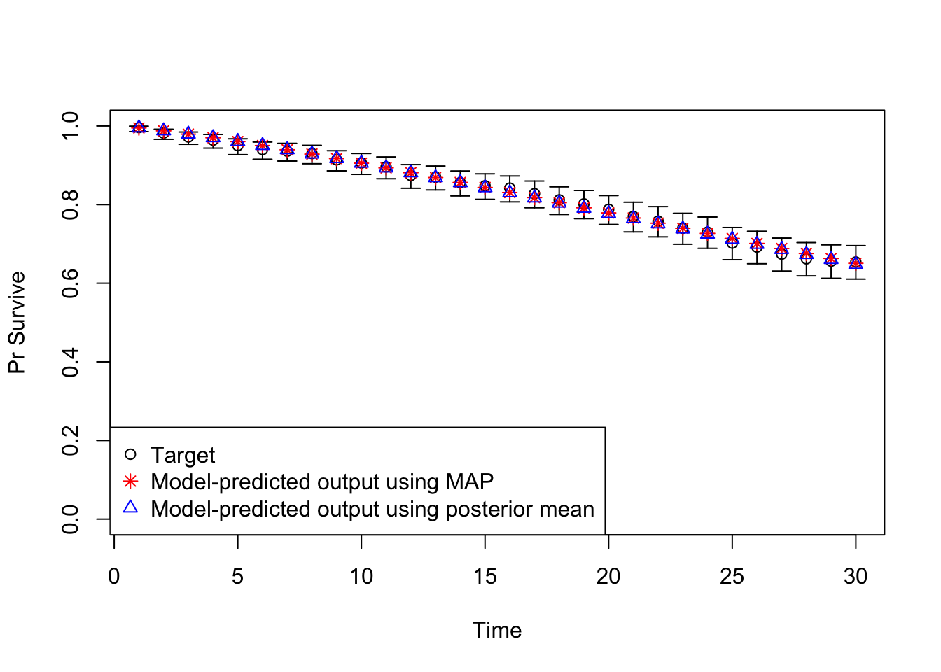
11 Plot model outputs vs targets (Prev)
# Plot: TARGET 2: Prevalence
plotrix::plotCI(x = lst_targets$Prev$time,
                y = lst_targets$Prev$value,
                ui = lst_targets$Prev$ub,
                li = lst_targets$Prev$lb,
                ylim = c(0, 1),
                xlab = "Time",
                ylab = "Prev")

points(x = lst_targets$Prev$time,
       y = v_out_map$Prev,
       pch = 8, col = "red")

points(x = lst_targets$Prev$time,
       y = v_out_post_mean$Prev,
       pch = 2, col = "blue")

legend("topright",
       legend = c("Target",
                  "Model-predicted output using MAP",
                  "Model-predicted output using posterior mean"),
       col = c("black", "red", "blue"),
       pch = c(1, 8, 2))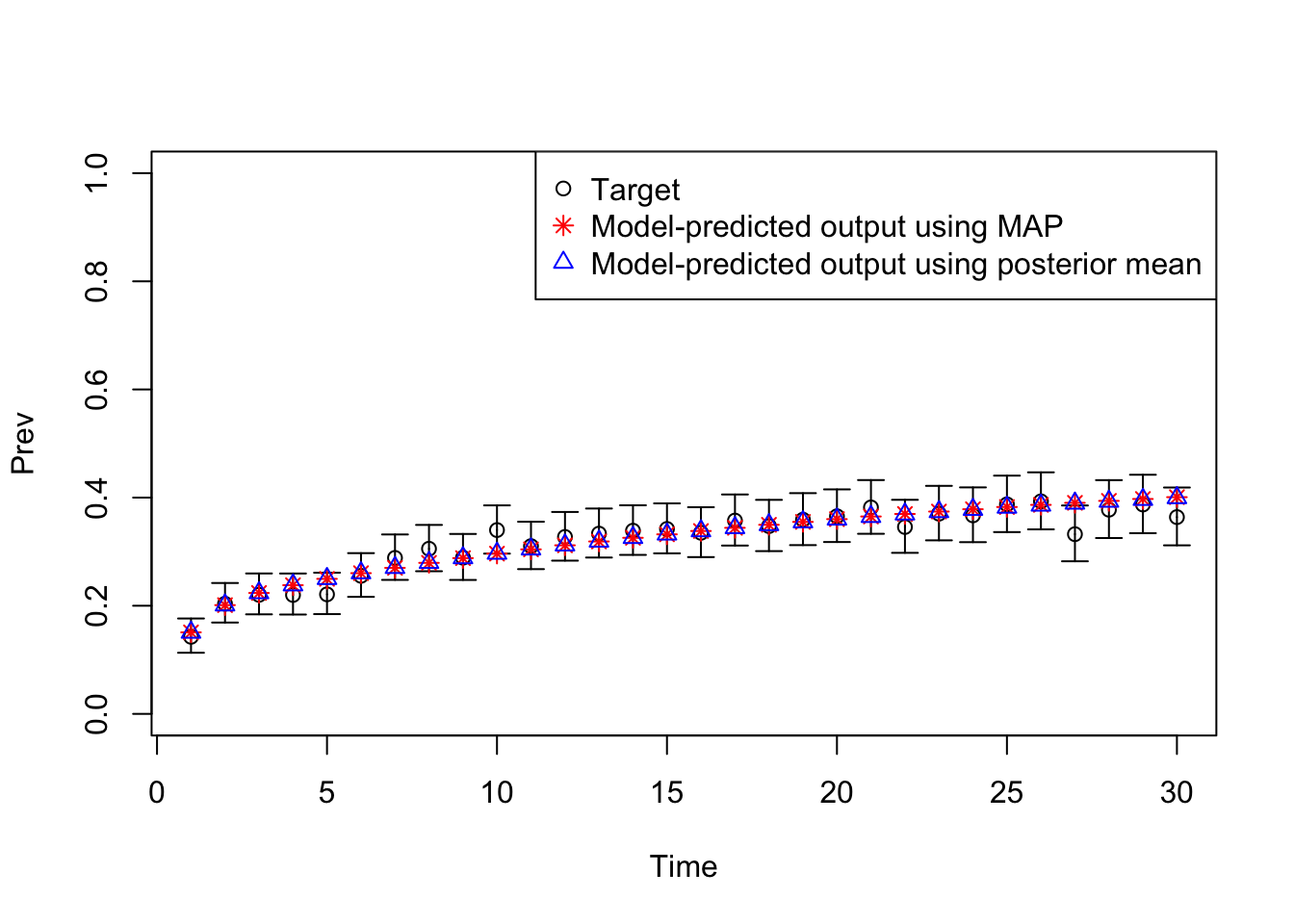
11 Plot model outputs vs targets (PropSick)
# Plot: TARGET 3: PropSick
plotrix::plotCI(x = lst_targets$PropSick$time,
                y = lst_targets$PropSick$value,
                ui = lst_targets$PropSick$ub,
                li = lst_targets$PropSick$lb,
                ylim = c(0, 1),
                xlab = "Time",
                ylab = "PropSick")

points(x = lst_targets$PropSick$time,
       y = v_out_map$PropSick,
       pch = 8, col = "red")

points(x = lst_targets$PropSick$time,
       y = v_out_post_mean$PropSick,
       pch = 2, col = "blue")

legend("topright",
       legend = c("Target",
                  "Model-predicted output using MAP",
                  "Model-predicted output using posterior mean"),
       col = c("black", "red", "blue"),
       pch = c(1, 8, 2))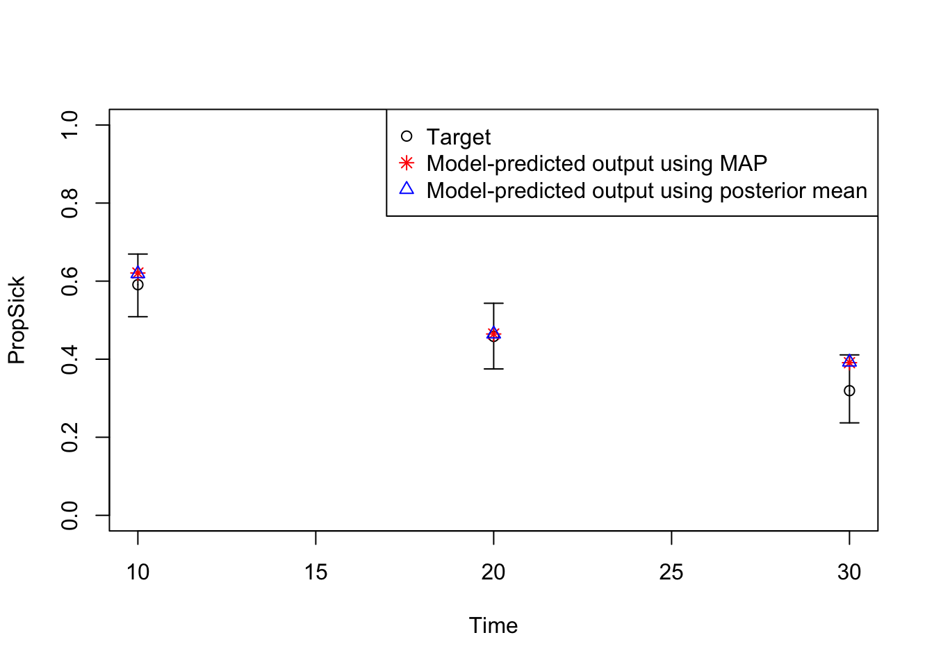
10.05 Advanced visualization: pairwise correlations
gg_post_pairs_corr <- GGally::ggpairs(
  data.frame(m_calib_res[, v_param_names]),
  upper = list(continuous = wrap("cor",
                                 color = "black",
                                 size = 5)),
  diag = list(continuous = wrap("barDiag",
                                alpha = 0.8)),
  lower = list(continuous = wrap("points",
                                 alpha = 0.3,
                                 size = 0.7)),
  columnLabels = v_param_names
) +
  theme_bw(base_size = 18) +
  theme(axis.title.x = element_blank(),
        axis.text.x = element_text(size = 14),
        axis.title.y = element_blank(),
        axis.text.y = element_blank(),
        axis.ticks.y = element_blank(),
        strip.background = element_rect(fill = "white",
                                        color = "white"),
        strip.text = element_text(hjust = 0))
gg_post_pairs_corr
`stat_bin()` using `bins = 30`. Pick better value `binwidth`.
`stat_bin()` using `bins = 30`. Pick better value `binwidth`.
`stat_bin()` using `bins = 30`. Pick better value `binwidth`.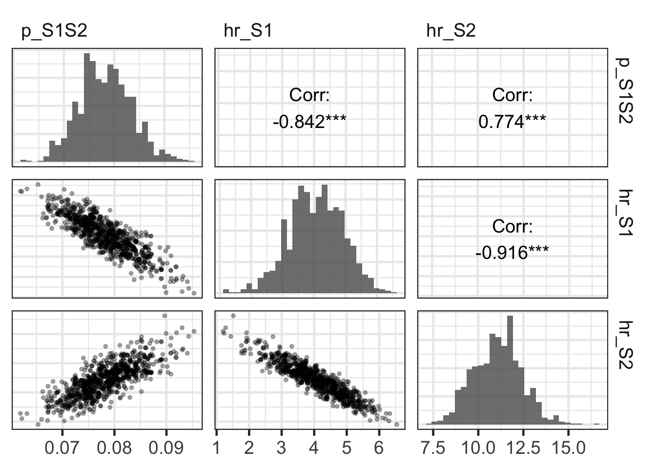
10.06 Prior vs posterior comparison
# Sample from prior
m_samp_prior <- sample.prior(n_resamp)

# Prepare data for plotting
df_samp_prior <- reshape2::melt(
  cbind(PDF = "Prior", as.data.frame(m_samp_prior)),
  variable.name = "Parameter"
)
Using PDF as id variablesdf_samp_post_imis <- reshape2::melt(
cbind(PDF = "Posterior IMIS",
as.data.frame(m_calib_res[, v_param_names])),
variable.name = "Parameter"
)Using PDF as id variablesdf_samp_prior_post <- dplyr::bind_rows(df_samp_prior, df_samp_post_imis)
# Plot prior vs posterior
gg_prior_post_imis <- ggplot(df_samp_prior_post,
aes(x = value, y = ..density.., fill = PDF)) +
facet_wrap(~Parameter, scales = "free",
ncol = 4,
labeller = label_parsed) +
scale_x_continuous(n.breaks = 6) +
geom_density(alpha = 0.5) +
theme_bw(base_size = 16) +
theme(legend.position = "bottom",
axis.title.x = element_blank(),
axis.title.y = element_blank(),
axis.text.y = element_blank(),
axis.ticks.y = element_blank())
gg_prior_post_imisWarning: The dot-dot notation (`..density..`) was deprecated in ggplot2 3.4.0.
ℹ Please use `after_stat(density)` instead.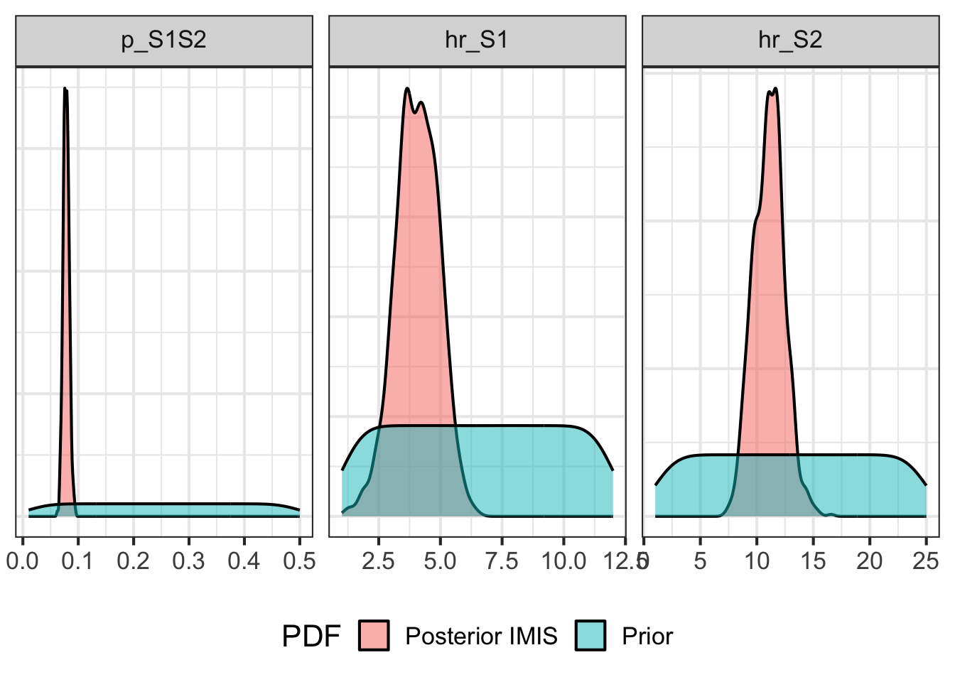
12 Propagate parameter uncertainty
### 11.01 Initialize output matrices  ------------------------------------------
m_out_surv     <- matrix(NA,
                         nrow = n_resamp,
                         ncol = length(lst_targets$Surv$value))

m_out_prev     <- matrix(NA,
                         nrow = n_resamp,
                         ncol = length(lst_targets$Prev$value))

m_out_propsick <- matrix(NA,
                         nrow = n_resamp,
                         ncol = length(lst_targets$PropSick$value))

### 11.02 Run model for each posterior parameter set  --------------------------
for (i in 1:n_resamp) { # i = 1
  model_res_temp <- run_sick_sicker_markov(m_calib_res[i, 1:3])
  m_out_surv[i, ] <- model_res_temp$Surv
  m_out_prev[i, ] <- model_res_temp$Prev
  m_out_propsick[i, ] <- model_res_temp$PropSick

  # Progress indicator
  if (i/100 == round(i/100, 0)) {
    cat('\r', paste(i/n_resamp * 100, "% done", sep = ""))
  }
}
 10% done
 20% done
 30% done
 40% done
 50% done
 60% done
 70% done
 80% done
 90% done
 100% done
### 11.03 Calculate posterior-predicted mean ----------------------------------
v_out_surv_post_mean <- colMeans(m_out_surv)
v_out_prev_post_mean <- colMeans(m_out_prev)
v_out_propsick_post_mean <- colMeans(m_out_propsick)
### 11.04 Calculate posterior-predicted 95% credible interval -----------------
m_out_surv_95cri <- colQuantiles(m_out_surv, probs = c(0.025, 0.975))
m_out_prev_95cri <- colQuantiles(m_out_prev, probs = c(0.025, 0.975))
m_out_propsick_95cri <- colQuantiles(m_out_propsick, probs = c(0.025, 0.975))
### 11.05 Prepare data for plotting -------------------------------------------
df_out_post <- data.frame(
Type = "Model output",
dplyr::bind_rows(
bind_cols(Outcome = "Survival",
time = lst_targets[[1]]$time,
value = v_out_surv_post_mean,
lb = m_out_surv_95cri[, 1],
ub = m_out_surv_95cri[, 2]),
bind_cols(Outcome = "Prevalence",
time = lst_targets[[2]]$time,
value = v_out_prev_post_mean,
lb = m_out_prev_95cri[, 1],
ub = m_out_prev_95cri[, 2]),
bind_cols(Outcome = "Proportion sick",
time = lst_targets[[3]]$time,
value = v_out_propsick_post_mean,
lb = m_out_propsick_95cri[, 1],
ub = m_out_propsick_95cri[, 2])
)
)
df_out_post$Outcome <- ordered(df_out_post$Outcome,
levels = c("Survival",
"Prevalence",
"Proportion sick"))
### 11.06 Plot targets vs model-predicted output ------------------------------
df_targets <- data.frame(
dplyr::bind_rows(
cbind(Type = "Target",
Outcome = "Survival",
lst_targets[[1]]),
cbind(Type = "Target",
Outcome = "Prevalence",
lst_targets[[2]]),
cbind(Type = "Target",
Outcome = "Proportion sick",
lst_targets[[3]])
)
)
df_targets$Outcome <- ordered(df_targets$Outcome,
levels = c("Survival",
"Prevalence",
"Proportion sick"))
ggplot(df_targets, aes(x = time, y = value, ymin = lb, ymax = ub)) +
geom_errorbar() +
geom_line(data = df_out_post,
aes(x = time, y = value),
col = "blue") +
geom_ribbon(data = df_out_post,
aes(ymin = lb, ymax = ub),
alpha = 0.4,
fill = "blue") +
facet_wrap(~ Outcome, scales = "free_x") +
scale_x_continuous("Time", n.breaks = 8) +
scale_y_continuous("Proportion", n.breaks = 8) +
theme_bw(base_size = 16)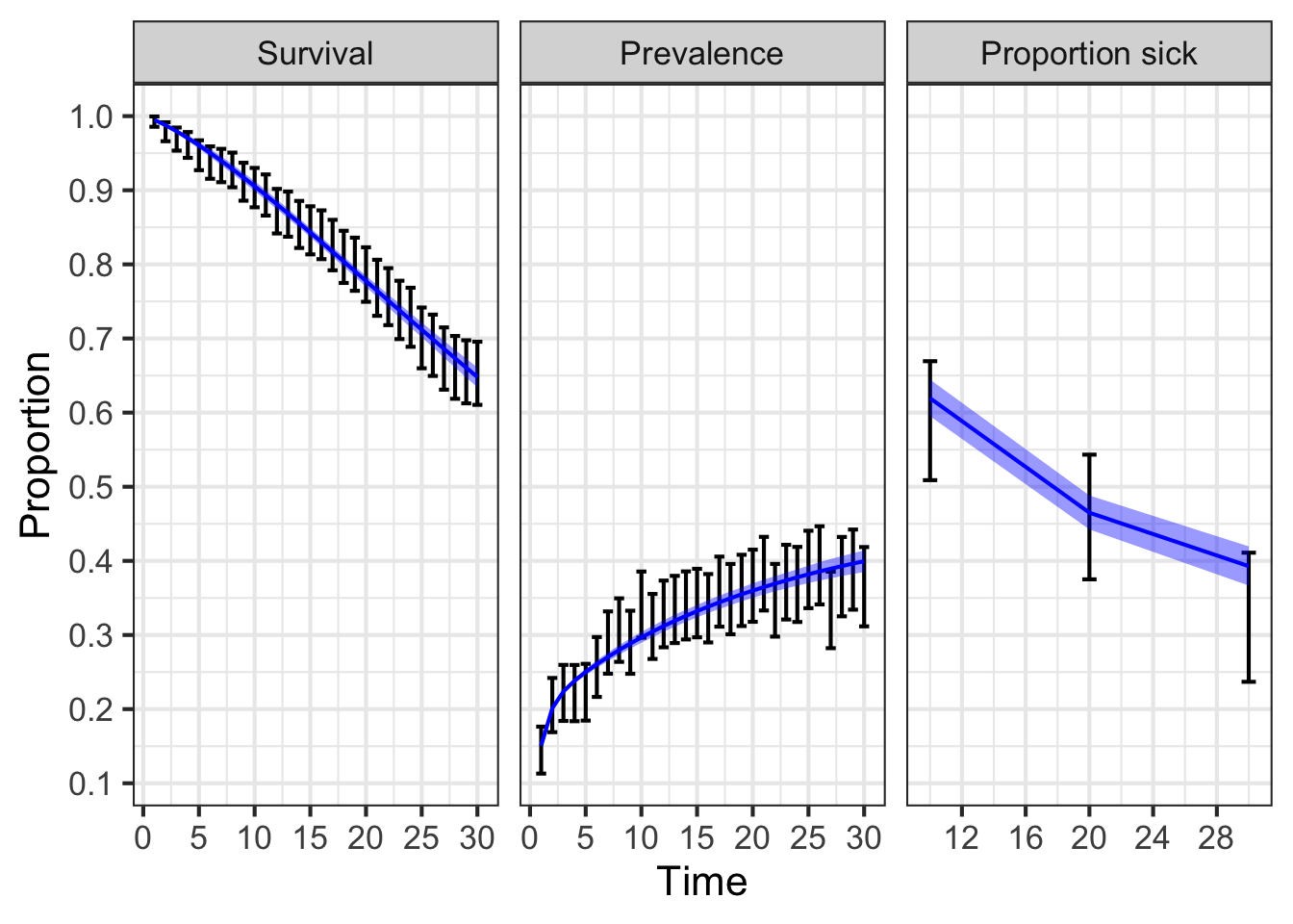
Note: This is a demonstration calibration exercise. In practice, calibration targets would be derived from high-quality epidemiological data, and more sophisticated goodness-of-fit measures might be employed depending on the data structure and modeling objectives.