# Load required packages
library(dplyr)
library(tidyr)
library(ggplot2)
library(scales)
library(diagram)
library(dampack)

# Install darthtools if needed
if (!require("darthtools")) {
  if (!require("devtools")) install.packages("devtools")
  devtools::install_github("DARTH-git/darthtools")
}
library(darthtools)

# Model structure
cycle_length <- 1   # Annual cycles
n_age_init   <- 25  # Starting age
n_age_max    <- 100 # Maximum age
n_cycles <- (n_age_max - n_age_init) / cycle_length3.- Sick-Sicker Time-Independent Model Exercise - Solutions
Overview
This document provides the complete solution to the Sick-Sicker model exercise. The exercise implements a time-independent cohort state-transition model to evaluate the cost-effectiveness of Strategy AB compared to Standard of Care.
Disease Description
The Sick-Sicker model represents a hypothetical disease affecting individuals starting at age 25, with:
- Four health states: Healthy (H), Sick (S1), Sicker (S2), and Dead (D)
- Natural history: Healthy individuals can become Sick, Sick individuals can recover, progress to Sicker, or die
- Key constraint: Sicker individuals cannot recover
- Follow-up period: Until age 100
Treatment Strategies
Standard of Care (SoC): Best available care reflecting natural disease progression
Strategy AB: Combination treatment providing: - 40% reduction in disease progression (HR = 0.6) - Improved quality of life in Sick state (utility 0.95 vs 0.75) - Additional annual cost of $25,000
Model Parameters
General Setup
Health States and Strategies
# Health states
v_names_states <- c("Healthy", "Sick", "Sicker", "Dead")
n_states <- length(v_names_states)

# Strategies
v_names_str <- c("Standard of care", "Strategy AB")
n_str <- length(v_names_str)

# Discounting
d_c <- 0.03  # Costs
d_e <- 0.03  # QALYs
Transition Parameters
# Annual transition rates
r_HD    <- 0.002  # Healthy to Dead (all-cause mortality)
r_HS1   <- 0.15   # Healthy to Sick
r_S1H   <- 0.5    # Sick to Healthy (recovery)
r_S1S2  <- 0.105  # Sick to Sicker (progression)

# Hazard ratios for mortality
hr_S1   <- 3   # Sick vs Healthy
hr_S2   <- 10  # Sicker vs Healthy

# Treatment effectiveness
hr_S1S2_trtAB <- 0.6  # Progression reduction under Strategy AB
Cost and Utility Parameters
# Annual costs
c_H     <- 2000   # Healthy
c_S1    <- 4000   # Sick
c_S2    <- 15000  # Sicker
c_D     <- 0      # Dead
c_trtAB <- 25000  # Treatment AB

# Annual utilities
u_H     <- 1.00   # Healthy
u_S1    <- 0.75   # Sick
u_S2    <- 0.50   # Sicker
u_D     <- 0.00   # Dead
u_trtAB <- 0.95   # Sick with treatment AB
Model Implementation
Process Model Inputs
# Within-cycle correction using Simpson's 1/3 rule
v_wcc <- gen_wcc(n_cycles = n_cycles, method = "Simpson1/3")

# Discount weights
v_dwc <- 1 / ((1 + (d_c * cycle_length)) ^ (0:n_cycles))
v_dwe <- 1 / ((1 + (d_e * cycle_length)) ^ (0:n_cycles))

# Calculate mortality rates
r_S1D <- r_HD * hr_S1  # Sick state mortality
r_S2D <- r_HD * hr_S2  # Sicker state mortality

# Convert rates to probabilities
p_HS1   <- rate_to_prob(r = r_HS1,  t = cycle_length)
p_S1H   <- rate_to_prob(r = r_S1H,  t = cycle_length)
p_S1S2  <- rate_to_prob(r = r_S1S2, t = cycle_length)
p_HD    <- rate_to_prob(r = r_HD,   t = cycle_length)
p_S1D   <- rate_to_prob(r = r_S1D,  t = cycle_length)
p_S2D   <- rate_to_prob(r = r_S2D,  t = cycle_length)

# Strategy AB: reduced progression probability
r_S1S2_trtAB <- r_S1S2 * hr_S1S2_trtAB
p_S1S2_trtAB <- rate_to_prob(r = r_S1S2_trtAB, t = cycle_length)
Initialize Cohort Traces
# Initial state vector (all start Healthy)
v_m_init <- c(Healthy = 1, Sick = 0, Sicker = 0, Dead = 0)

# Initialize cohort trace matrices
m_M <- matrix(NA,
              nrow = (n_cycles + 1),
              ncol = n_states,
              dimnames = list(0:n_cycles, v_names_states))
m_M[1, ] <- v_m_init

# Strategy AB trace (same structure)
m_M_strAB <- m_M
Create Transition Probability Matrices
# Standard of Care transition matrix
m_P <- matrix(0,
              nrow = n_states,
              ncol = n_states,
              dimnames = list(v_names_states, v_names_states))

# From Healthy
m_P["Healthy", "Healthy"] <- (1 - p_HD) * (1 - p_HS1)
m_P["Healthy", "Sick"]    <- (1 - p_HD) * p_HS1
m_P["Healthy", "Dead"]    <- p_HD

# From Sick
m_P["Sick", "Healthy"] <- (1 - p_S1D) * p_S1H
m_P["Sick", "Sick"]    <- (1 - p_S1D) * (1 - (p_S1H + p_S1S2))
m_P["Sick", "Sicker"]  <- (1 - p_S1D) * p_S1S2
m_P["Sick", "Dead"]    <- p_S1D

# From Sicker
m_P["Sicker", "Sicker"] <- 1 - p_S2D
m_P["Sicker", "Dead"]   <- p_S2D

# From Dead
m_P["Dead", "Dead"] <- 1

# Strategy AB transition matrix (modified progression)
m_P_strAB <- m_P
m_P_strAB["Sick", "Sick"]   <- (1 - p_S1D) * (1 - (p_S1H + p_S1S2_trtAB))
m_P_strAB["Sick", "Sicker"] <- (1 - p_S1D) * p_S1S2_trtAB

# Validate matrices
check_transition_probability(m_P, verbose = TRUE)
[1] "Valid transition probabilities"check_transition_probability(m_P_strAB, verbose = TRUE)[1] "Valid transition probabilities"check_sum_of_transition_array(m_P, n_states = n_states,
n_cycles = n_cycles, verbose = TRUE)[1] "This is a valid transition matrix"check_sum_of_transition_array(m_P_strAB, n_states = n_states,
n_cycles = n_cycles, verbose = TRUE)[1] "This is a valid transition matrix"Run Markov Model
# Simulate cohort over time
for (t in 1:n_cycles) {
  m_M[t + 1, ]       <- m_M[t, ] %*% m_P
  m_M_strAB[t + 1, ] <- m_M_strAB[t, ] %*% m_P_strAB
}

# Store traces in list
l_m_M <- list(m_M, m_M_strAB)
names(l_m_M) <- v_names_str
Results
Cohort Trace Visualization
# Prepare data for plotting
df_M <- data.frame(Cycle = 0:n_cycles, m_M)
df_M_strAB <- data.frame(Cycle = 0:n_cycles, m_M_strAB)

# Convert to long format
df_M_long <- tidyr::gather(df_M, key = "Health_State", value = "Proportion", -Cycle)
df_M_strAB_long <- tidyr::gather(df_M_strAB, key = "Health_State", value = "Proportion", -Cycle)

# Add strategy labels
df_M_long$Strategy <- "Standard of Care"
df_M_strAB_long$Strategy <- "Strategy AB"

# Combine
df_combined <- rbind(df_M_long, df_M_strAB_long)

# Plot
ggplot(df_combined, aes(x = Cycle, y = Proportion,
                        color = Health_State, linetype = Health_State)) +
  geom_line(size = 1) +
  facet_wrap(~ Strategy) +
  scale_x_continuous(breaks = seq(0, n_cycles, by = 10)) +
  labs(title = "Cohort Trace: Standard of Care vs Strategy AB",
       x = "Cycle (Years)",
       y = "Proportion of Cohort",
       color = "Health State",
       linetype = "Health State") +
  theme_minimal(base_size = 12) +
  theme(legend.position = "bottom")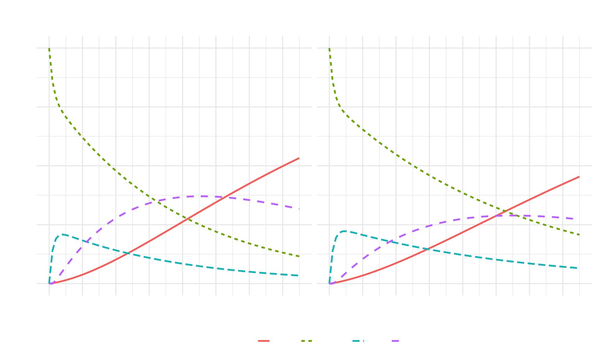
Interpretation: Strategy AB shows slower disease progression, with fewer individuals reaching the Sicker state and improved survival compared to Standard of Care.
Calculate Expected Outcomes
# State rewards for Standard of Care
v_u_SoC <- c(Healthy = u_H, Sick = u_S1, Sicker = u_S2, Dead = u_D) * cycle_length
v_c_SoC <- c(Healthy = c_H, Sick = c_S1, Sicker = c_S2, Dead = c_D) * cycle_length

# State rewards for Strategy AB
v_u_strAB <- c(Healthy = u_H, Sick = u_trtAB, Sicker = u_S2, Dead = u_D) * cycle_length
v_c_strAB <- c(Healthy = c_H, Sick = c_S1 + c_trtAB,
               Sicker = c_S2 + c_trtAB, Dead = c_D) * cycle_length

# Store in lists
l_u <- list(v_u_SoC, v_u_strAB)
l_c <- list(v_c_SoC, v_c_strAB)
names(l_u) <- names(l_c) <- v_names_str

# Calculate total QALYs and costs
v_tot_qaly <- v_tot_cost <- vector(mode = "numeric", length = n_str)
names(v_tot_qaly) <- names(v_tot_cost) <- v_names_str

for (i in 1:n_str) {
  v_qaly_str <- l_m_M[[i]] %*% l_u[[i]]
  v_cost_str <- l_m_M[[i]] %*% l_c[[i]]

  v_tot_qaly[i] <- t(v_qaly_str) %*% (v_dwe * v_wcc)
  v_tot_cost[i] <- t(v_cost_str) %*% (v_dwc * v_wcc)
}

# Display results
results_df <- data.frame(
  Strategy = v_names_str,
  Total_QALYs = round(v_tot_qaly, 2),
  Total_Costs = scales::dollar(v_tot_cost)
)
knitr::kable(results_df, caption = "Total Expected Outcomes by Strategy")| Strategy | Total_QALYs | Total_Costs | |
|---|---|---|---|
| Standard of care | Standard of care | 20.71 | $151,580 |
| Strategy AB | Strategy AB | 23.14 | $378,875 |
Cost-Effectiveness Analysis
# Calculate ICERs
df_cea <- calculate_icers(cost = v_tot_cost,
                          effect = v_tot_qaly,
                          strategies = v_names_str)

# Format CEA table
table_cea <- format_table_cea(df_cea)
knitr::kable(table_cea, caption = "Cost-Effectiveness Analysis Results")| Strategy | Costs (\() | QALYs|Incremental Costs (\)) | Incremental QALYs | ICER ($/QALY) | Status | |||
|---|---|---|---|---|---|---|---|
| Standard of care | Standard of care | 151,580 | 20.71 | NA | NA | NA | ND |
| Strategy AB | Strategy AB | 378,875 | 23.14 | 227,295 | 2.43 | 93,710 | ND |
Interpretation:
- Strategy AB provides additional QALYs at an additional cost
- The ICER represents the cost per additional QALY gained
- Decision-makers would compare this ICER to their willingness-to-pay threshold (commonly $50,000-$150,000/QALY in the US)
Cost-Effectiveness Plane
plot(df_cea, label = "all", txtsize = 12) +
  expand_limits(x = max(table_cea$QALYs) + 0.5) +
  labs(title = "Cost-Effectiveness Frontier",
       x = "Total QALYs",
       y = "Total Costs ($)") +
  theme_minimal(base_size = 12) +
  theme(legend.position = c(0.8, 0.3))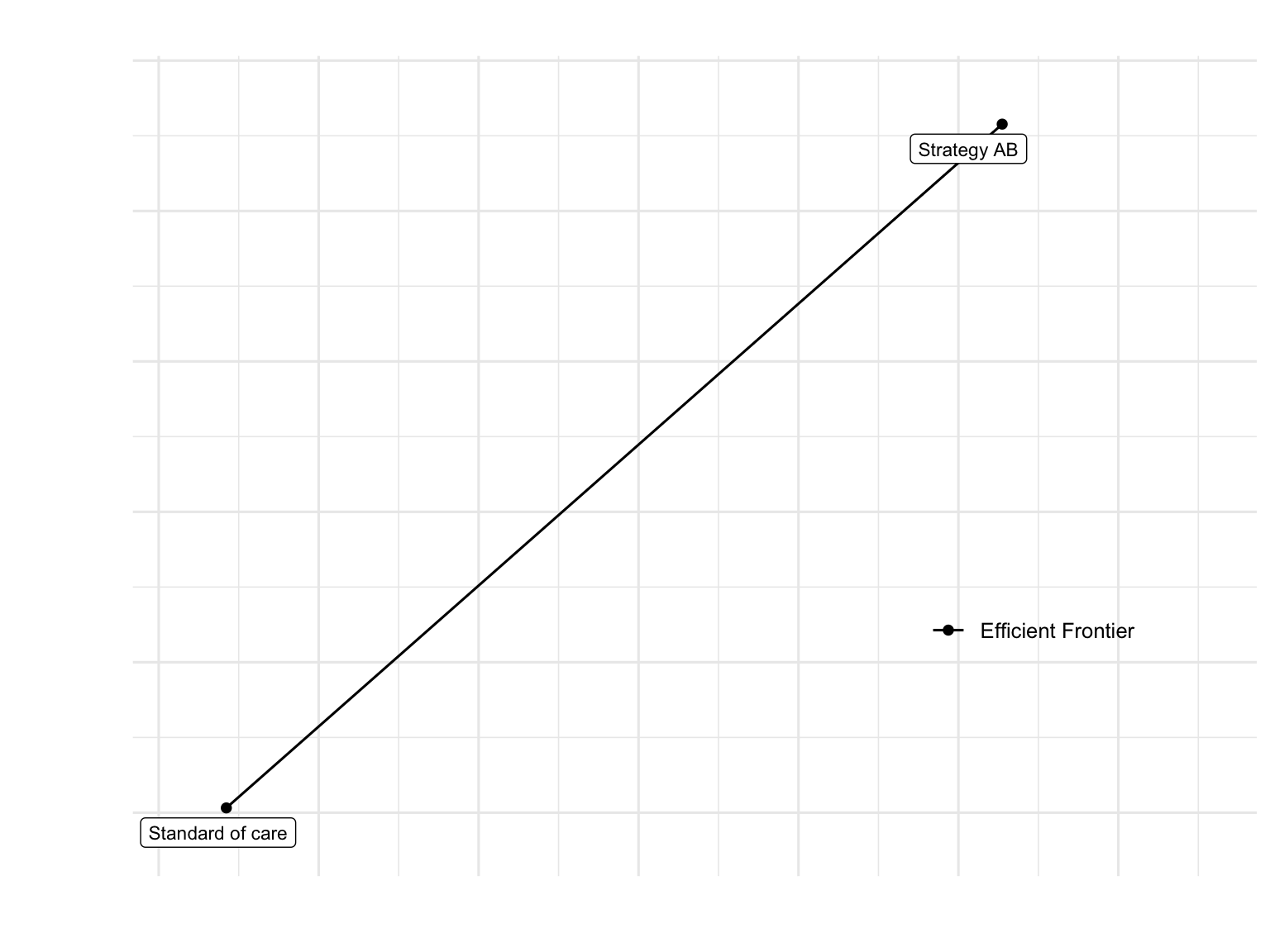
Conclusions
Clinical Effectiveness: Strategy AB successfully reduces disease progression and improves quality of life for Sick individuals
Economic Impact: The treatment adds substantial costs but provides meaningful health benefits
Cost-Effectiveness: The ICER indicates whether Strategy AB represents good value for money depends on the decision-maker’s willingness-to-pay threshold
Model Insights: The cohort trace shows clear differences in disease trajectories between strategies, with Strategy AB maintaining more individuals in better health states
References
This exercise is based on work by the Decision Analysis in R for Technologies in Health (DARTH) workgroup:
Alarid-Escudero F, Krijkamp EM, Enns EA, et al. A Need for Change! A Coding Framework for Improving Transparency in Decision Modeling. PharmacoEconomics 2019;37:1329-1339.
DARTH workgroup: http://darthworkgroup.com