# Load required packages
library(dplyr)
library(tidyr)
library(ggplot2)
library(scales)
library(diagram)
library(dampack)

# Install darthtools if needed
if (!require("darthtools")) {
  if (!require("devtools")) install.packages("devtools")
  devtools::install_github("DARTH-git/darthtools")
}
library(darthtools)

# Model structure
cycle_length <- 1   # Annual cycles
n_age_init   <- 25  # Starting age
n_age_max    <- 100 # Maximum age
n_cycles <- (n_age_max - n_age_init) / cycle_length4.- Sick-Sicker Time (Age)-Dependent Model Exercise - Solutions
Overview
This document provides the complete solution to the age-dependent Sick-Sicker model exercise. The exercise implements a simulation-time-dependent cohort state-transition model incorporating age-specific mortality to evaluate the cost-effectiveness of Strategy AB compared to Standard of Care.
Disease Description
The age-dependent Sick-Sicker model extends the basic model by incorporating:
- Age-specific mortality: Using real-world mortality data from the Human Mortality Database (HMD)
- Four health states: Healthy (H), Sick (S1), Sicker (S2), and Dead (D)
- Natural history: Same as basic model but with age-varying mortality risks
- Follow-up period: From age 25 until age 100
Treatment Strategies
Standard of Care (SoC): Best available care reflecting natural disease progression with age-dependent mortality
Strategy AB: Combination treatment providing: - 40% reduction in disease progression (HR = 0.6) - Improved quality of life in Sick state (utility 0.95 vs 0.75) - Additional annual cost of $25,000
Key Difference from Time-Independent Model
The critical enhancement is the use of age-specific mortality rates that vary across the time horizon, making the transition probabilities time-dependent.
Model Parameters
General Setup
Age Labels
# Create age labels for each cycle
v_age_names <- paste(rep(n_age_init:(n_age_max-1), each = 1/cycle_length),
                     1:(1/cycle_length),
                     sep = ".")
Health States and Strategies
# Health states
v_names_states <- c("H", "S1", "S2", "D")
n_states <- length(v_names_states)

# Strategies
v_names_str <- c("Standard of care", "Strategy AB")
n_str <- length(v_names_str)

# Discounting
d_c <- 0.03  # Costs
d_e <- 0.03  # QALYs

# Within-cycle correction using Simpson's 1/3 rule
v_wcc <- gen_wcc(n_cycles = n_cycles, method = "Simpson1/3")
Transition Parameters
# Annual transition rates (constant across age)
r_HS1  <- 0.15   # Healthy to Sick
r_S1H  <- 0.5    # Sick to Healthy (recovery)
r_S1S2 <- 0.105  # Sick to Sicker (progression)

# Hazard ratios for mortality (applied to age-specific baseline)
hr_S1  <- 3   # Sick vs Healthy
hr_S2  <- 10  # Sicker vs Healthy

# Treatment effectiveness
hr_S1S2_trtAB <- 0.6  # Progression reduction under Strategy AB
Cost and Utility Parameters
# Annual costs
c_H     <- 2000   # Healthy
c_S1    <- 4000   # Sick
c_S2    <- 15000  # Sicker
c_D     <- 0      # Dead
c_trtAB <- 25000  # Treatment AB

# Annual utilities
u_H     <- 1.00   # Healthy
u_S1    <- 0.75   # Sick
u_S2    <- 0.50   # Sicker
u_D     <- 0.00   # Dead
u_trtAB <- 0.95   # Sick with treatment AB
Load Age-Specific Mortality Data
# Load Human Mortality Database data for USA 2015
lt_usa_2015 <- read.csv("data/HMD_USA_Mx_2015.csv")

# Extract age-specific all-cause mortality rates
v_r_mort_by_age <- lt_usa_2015 %>%
  dplyr::filter(Age >= n_age_init & Age < n_age_max) %>%
  dplyr::select(Total) %>%
  as.matrix()

# Display first few mortality rates
head(v_r_mort_by_age, 10)
Total
[1,] 0.001014
[2,] 0.000999
[3,] 0.001070
[4,] 0.001087
[5,] 0.001162
[6,] 0.001167
[7,] 0.001213
[8,] 0.001289
[9,] 0.001331
[10,] 0.001375Note: These are annual mortality rates that increase with age, making the model more realistic than assuming constant mortality.
Process Model Inputs
# Discount weights
v_dwc <- 1 / ((1 + (d_c * cycle_length)) ^ (0:n_cycles))
v_dwe <- 1 / ((1 + (d_e * cycle_length)) ^ (0:n_cycles))

# Create age-specific mortality rate vector for all cycles
v_r_HD_age <- rep(v_r_mort_by_age, each = 1/cycle_length)
names(v_r_HD_age) <- v_age_names

# Calculate age-specific mortality rates for disease states
v_r_S1D_age <- v_r_HD_age * hr_S1  # Sick state mortality
v_r_S2D_age <- v_r_HD_age * hr_S2  # Sicker state mortality

# Convert rates to probabilities
p_HS1  <- rate_to_prob(r = r_HS1,  t = cycle_length)
p_S1H  <- rate_to_prob(r = r_S1H,  t = cycle_length)
p_S1S2 <- rate_to_prob(r = r_S1S2, t = cycle_length)

# Age-specific mortality probabilities
v_p_HD_age  <- rate_to_prob(v_r_HD_age,  t = cycle_length)
v_p_S1D_age <- rate_to_prob(v_r_S1D_age, t = cycle_length)
v_p_S2D_age <- rate_to_prob(v_r_S2D_age, t = cycle_length)

# Strategy AB: reduced progression probability
r_S1S2_trtAB <- r_S1S2 * hr_S1S2_trtAB
p_S1S2_trtAB <- rate_to_prob(r = r_S1S2_trtAB, t = cycle_length)
Model Implementation
Initialize Cohort Traces
# Initial state vector (all start Healthy)
v_m_init <- c(H = 1, S1 = 0, S2 = 0, D = 0)

# Initialize cohort trace matrices
m_M_SoC <- matrix(NA,
                  nrow = (n_cycles + 1),
                  ncol = n_states,
                  dimnames = list(0:n_cycles, v_names_states))
m_M_SoC[1, ] <- v_m_init

# Strategy AB trace (same structure)
m_M_strAB <- m_M_SoC
Create Transition Probability Arrays
Key Difference: Unlike the time-independent model with a single transition matrix, we now create a 3-dimensional array where each “slice” represents the transition probabilities for a specific cycle (age).
# Standard of Care transition probability array
# Dimensions: [from_state, to_state, cycle]
a_P_SoC <- array(0,
                 dim = c(n_states, n_states, n_cycles),
                 dimnames = list(v_names_states,
                                v_names_states,
                                0:(n_cycles - 1)))

# From Healthy
a_P_SoC["H", "H", ]  <- (1 - v_p_HD_age) * (1 - p_HS1)
a_P_SoC["H", "S1", ] <- (1 - v_p_HD_age) * p_HS1
a_P_SoC["H", "D", ]  <- v_p_HD_age

# From Sick
a_P_SoC["S1", "H", ]  <- (1 - v_p_S1D_age) * p_S1H
a_P_SoC["S1", "S1", ] <- (1 - v_p_S1D_age) * (1 - (p_S1H + p_S1S2))
a_P_SoC["S1", "S2", ] <- (1 - v_p_S1D_age) * p_S1S2
a_P_SoC["S1", "D", ]  <- v_p_S1D_age

# From Sicker
a_P_SoC["S2", "S2", ] <- 1 - v_p_S2D_age
a_P_SoC["S2", "D", ]  <- v_p_S2D_age

# From Dead
a_P_SoC["D", "D", ] <- 1

# Strategy AB transition probability array (modified progression)
a_P_strAB <- a_P_SoC
a_P_strAB["S1", "S1", ] <- (1 - v_p_S1D_age) * (1 - (p_S1H + p_S1S2_trtAB))
a_P_strAB["S1", "S2", ] <- (1 - v_p_S1D_age) * p_S1S2_trtAB

# Validate arrays
check_transition_probability(a_P_SoC, verbose = TRUE)
[1] "Valid transition probabilities"check_transition_probability(a_P_strAB, verbose = TRUE)[1] "Valid transition probabilities"check_sum_of_transition_array(a_P_SoC, n_states = n_states,
n_cycles = n_cycles, verbose = TRUE)[1] "This is a valid transition array"check_sum_of_transition_array(a_P_strAB, n_states = n_states,
n_cycles = n_cycles, verbose = TRUE)[1] "This is a valid transition array"Run Markov Model
Key Difference: The loop now uses a different transition matrix for each cycle based on the cohort’s age.
# Simulate cohort over time with age-dependent transitions
for(t in 1:n_cycles) {
  # Use the transition matrix for cycle t (age-specific)
  m_M_SoC[t + 1, ]   <- m_M_SoC[t, ]   %*% a_P_SoC[, , t]
  m_M_strAB[t + 1, ] <- m_M_strAB[t, ] %*% a_P_strAB[, , t]
}

# Store traces in list
l_m_M <- list(m_M_SoC, m_M_strAB)
names(l_m_M) <- v_names_str
Results
# Create data frame for plotting
df_mortality <- data.frame(
  Age     = n_age_init:(n_age_max - 1),
  Healthy = as.numeric(v_r_mort_by_age),
  Sick    = as.numeric(v_r_mort_by_age) * hr_S1,
  Sicker  = as.numeric(v_r_mort_by_age) * hr_S2
)


# Convert to long format
df_mortality_long <- tidyr::gather(df_mortality, key = "State", value = "Rate", -Age)

# Plot
ggplot(df_mortality_long, aes(x = Age, y = Rate, color = State)) +
  geom_line(size = 1) +
  scale_y_log10() +
  labs(title = "Age-Specific Mortality Rates by Health State",
       x = "Age (years)",
       y = "Annual Mortality Rate (log scale)",
       color = "Health State") +
  theme_minimal(base_size = 12) +
  theme(
    legend.position = "bottom")
Visualize Age-Specific Mortality Rates

Interpretation: Mortality rates increase exponentially with age and are substantially higher in disease states due to the hazard ratios.
Cohort Trace Visualization
# Prepare data for plotting
df_M_SoC <- data.frame(Cycle = 0:n_cycles, m_M_SoC, check.names = FALSE)
df_M_strAB <- data.frame(Cycle = 0:n_cycles, m_M_strAB, check.names = FALSE)

# Convert to long format
df_M_SoC_long <- tidyr::gather(df_M_SoC, key = "Health_State", value = "Proportion", -Cycle)
df_M_strAB_long <- tidyr::gather(df_M_strAB, key = "Health_State", value = "Proportion", -Cycle)

# Rename health states
df_M_SoC_long$Health_State <- factor(
  df_M_SoC_long$Health_State,
  levels = c("H", "S1", "S2", "D"),
  labels = c("Healthy", "Sick", "Sicker", "Dead")
)

df_M_strAB_long$Health_State <- factor(
  df_M_strAB_long$Health_State,
  levels = c("H", "S1", "S2", "D"),
  labels = c("Healthy", "Sick", "Sicker", "Dead")
)

# Add strategy labels
df_M_SoC_long$Strategy <- "Standard of Care"
df_M_strAB_long$Strategy <- "Strategy AB"

# Combine
df_combined <- rbind(df_M_SoC_long, df_M_strAB_long)

# Plot
ggplot(df_combined, aes(x = Cycle, y = Proportion,
                        color = Health_State, linetype = Health_State)) +
  geom_line(size = 1) +
  facet_wrap(~ Strategy) +
  scale_x_continuous(breaks = seq(0, n_cycles, by = 10)) +
  labs(title = "Cohort Trace: Standard of Care vs Strategy AB (Age-Dependent)",
       x = "Cycle (Years from Age 25)",
       y = "Proportion of Cohort",
       color = "Health State",
       linetype = "Health State") +
  theme_minimal(base_size = 12) +
  theme(legend.position = "bottom")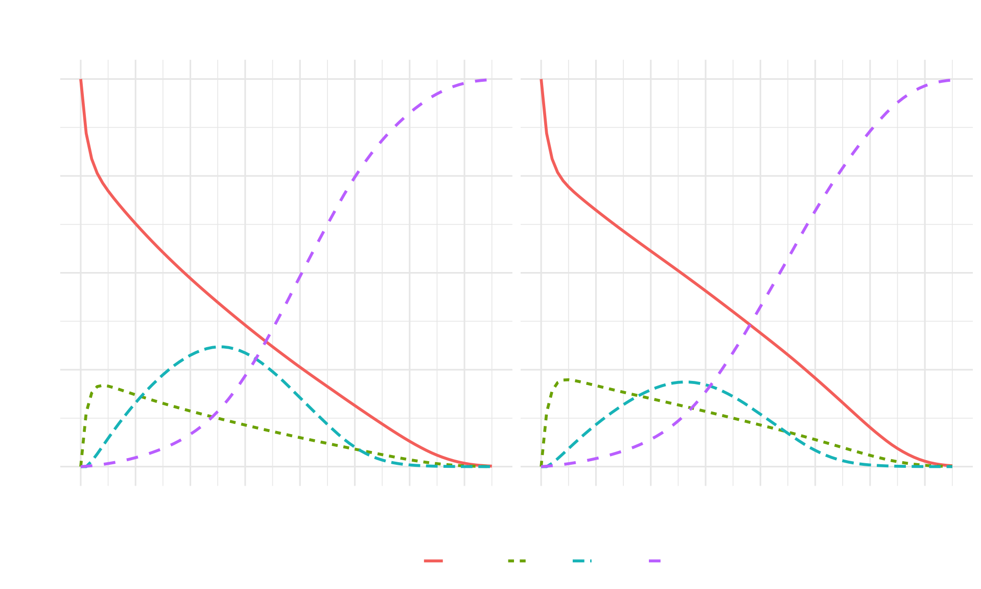
Interpretation:
- The Dead state accumulates faster than in the time-independent model due to increasing age-specific mortality
- Strategy AB still shows benefits in slowing disease progression
- The impact of age-dependent mortality becomes more pronounced in later cycles
- Both strategies show eventual convergence to 100% in the Dead state as the cohort ages
Calculate Expected Outcomes
# State rewards for Standard of Care
v_u_SoC <- c(H = u_H, S1 = u_S1, S2 = u_S2, D = u_D) * cycle_length
v_c_SoC <- c(H = c_H, S1 = c_S1, S2 = c_S2, D = c_D) * cycle_length

# State rewards for Strategy AB
v_u_strAB <- c(H = u_H, S1 = u_trtAB, S2 = u_S2, D = u_D) * cycle_length
v_c_strAB <- c(H = c_H, S1 = c_S1 + c_trtAB,
               S2 = c_S2 + c_trtAB, D = c_D) * cycle_length

# Store in lists
l_u <- list(v_u_SoC, v_u_strAB)
l_c <- list(v_c_SoC, v_c_strAB)
names(l_u) <- names(l_c) <- v_names_str

# Calculate total QALYs and costs
v_tot_qaly <- v_tot_cost <- vector(mode = "numeric", length = n_str)
names(v_tot_qaly) <- names(v_tot_cost) <- v_names_str

for (i in 1:n_str) {
  v_qaly_str <- l_m_M[[i]] %*% l_u[[i]]
  v_cost_str <- l_m_M[[i]] %*% l_c[[i]]

  v_tot_qaly[i] <- t(v_qaly_str) %*% (v_dwe * v_wcc)
  v_tot_cost[i] <- t(v_cost_str) %*% (v_dwc * v_wcc)
}

# Display results
results_df <- data.frame(
  Strategy = v_names_str,
  Total_QALYs = round(v_tot_qaly, 2),
  Total_Costs = scales::dollar(v_tot_cost)
)
knitr::kable(results_df, caption = "Total Expected Outcomes by Strategy (Age-Dependent Model)")| Strategy | Total_QALYs | Total_Costs | |
|---|---|---|---|
| Standard of care | Standard of care | 18.90 | $113,790 |
| Strategy AB | Strategy AB | 21.12 | $293,561 |
Comparison to Time-Independent Model:
- Total QALYs are likely lower due to more realistic age-dependent mortality
- Cost differences may vary due to shorter survival in disease states
- The age-dependent model provides more accurate estimates for decision-making
Cost-Effectiveness Analysis
# Calculate ICERs
df_cea <- calculate_icers(cost = v_tot_cost,
                          effect = v_tot_qaly,
                          strategies = v_names_str)

# Format CEA table
table_cea <- format_table_cea(df_cea)
knitr::kable(table_cea, caption = "Cost-Effectiveness Analysis Results (Age-Dependent Model)")| Strategy | Costs (\() | QALYs|Incremental Costs (\)) | Incremental QALYs | ICER ($/QALY) | Status | |||
|---|---|---|---|---|---|---|---|
| Standard of care | Standard of care | 113,790 | 18.90 | NA | NA | NA | ND |
| Strategy AB | Strategy AB | 293,561 | 21.12 | 179,771 | 2.22 | 81,002 | ND |
Interpretation:
- The ICER may differ from the time-independent model
- Age-dependent mortality affects both survival and time spent in each state
- This more realistic model provides better estimates for policy decisions
Cost-Effectiveness Plane
Cost-Effectiveness Plane
plot(df_cea, label = "all", txtsize = 12) +
  expand_limits(x = max(table_cea$QALYs) + 0.5) +
  labs(title = "Cost-Effectiveness Frontier (Age-Dependent Model)",
       x = "Total QALYs",
       y = "Total Costs ($)") +
  theme_minimal(base_size = 12) +
  theme(legend.position = c(0.8, 0.3))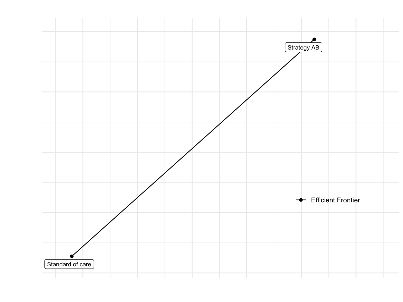
Model Comparison: Time-Independent vs Age-Dependent
Key Differences
- Mortality Assumptions:
- Time-independent: Constant mortality rates
- Age-dependent: Realistic age-varying mortality from HMD data
- Model Structure:
- Time-independent: Single transition probability matrix
- Age-dependent: Array of matrices (one per cycle/age)
- Computational Complexity:
- Time-independent: Simpler, faster computation
- Age-dependent: More realistic but computationally intensive
- Results Accuracy:
- Time-independent: Good for teaching, may overestimate survival
- Age-dependent: More accurate for real-world decision-making
When to Use Each Model
Time-Independent: - Teaching and learning concepts - Diseases with negligible age effects - Preliminary analyses - Sensitivity analyses where age effects are constant
Age-Dependent: - Diseases affecting older populations - Long time horizons - Final analyses for policy decisions - When accurate life expectancy estimates are critical
Conclusions
Model Realism: Incorporating age-dependent mortality provides more accurate survival estimates and better reflects real-world disease progression
Clinical Effectiveness: Strategy AB maintains its benefits in reducing disease progression even with realistic mortality patterns
Economic Impact: The treatment’s value proposition is evaluated more accurately when accounting for age-varying baseline risk
Policy Implications: Age-dependent models are essential for informed healthcare decision-making, especially for chronic diseases affecting aging populations
Technical Implementation: The transition from matrices to arrays is straightforward but requires careful indexing and validation
References
This exercise is based on work by the Decision Analysis in R for Technologies in Health (DARTH) workgroup:
Alarid-Escudero F, Krijkamp EM, Enns EA, et al. A Need for Change! A Coding Framework for Improving Transparency in Decision Modeling. PharmacoEconomics 2019;37:1329-1339.
Alarid-Escudero F, Krijkamp E, Enns EA, et al. An Introductory Tutorial on Cohort State-Transition Models in R Using a Cost-Effectiveness Analysis Example. Medical Decision Making 2023;43(1):3-20.
Alarid-Escudero F, Krijkamp E, Enns EA, et al. A Tutorial on Time-Dependent Cohort State-Transition Models in R using a Cost-Effectiveness Analysis Example. Medical Decision Making 2023;43(1):21-41.
DARTH workgroup: http://darthworkgroup.com
Mortality Data Source: Human Mortality Database. University of California, Berkeley (USA), and Max Planck Institute for Demographic Research (Germany). Available at www.mortality.org